Transcription
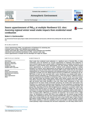
Atmospheric Environment 142 (2016) 210e219Contents lists available at ScienceDirectAtmospheric Environmentjournal homepage: www.elsevier.com/locate/atmosenvSource apportionment of PM2.5 at multiple Northwest U.S. sites:Assessing regional winter wood smoke impacts from residential woodcombustionRobert A. KotchenrutherU.S. Environmental Protection Agency Region 10, Office of Environmental Review and Assessment, 1200 Sixth Avenue, Mailstop OEA-140, Seattle, WA, 98101,USAh i g h l i g h t s Source apportionment of PM2.5 was performed on 19 Northwest U.S. monitoring sites. Common sources of PM2.5 were identified across multiple sites. Winter wood smoke PM2.5 impacts from residential wood combustion were quantified. Residential wood combustion contributions to PM2.5 spanned a wide range. Source apportionment at multiple sites has advantages over single site analysis.a r t i c l e i n f oa b s t r a c tArticle history:Received 12 April 2016Received in revised form20 July 2016Accepted 23 July 2016Available online 25 July 2016Wood smoke from residential wood combustion is a significant source of elevated PM2.5 in manycommunities across the Northwest U.S. Accurate representation of residential wood combustion insource-oriented regional scale air quality models is challenging because of multiple uncertainties. As analternative to source-oriented source apportionment, this work provides, through receptor-orientedsource apportionment, an assessment of winter residential wood combustion impacts at multipleNorthwest U.S. locations. Source apportionment was performed on chemically speciated PM2.5 from 19monitoring sites using the Positive Matrix Factorization (PMF) receptor model. Each site was modeledindependently, but a common data preparation and modeling protocol was used so that results were ascomparable as possible across sites. Model solutions had from 4 to 8 PMF factors, depending on the site.PMF factors at each site were associated with a source classification (e.g., primary wood smoke), adominant chemical composition (e.g., ammonium nitrate), or were some mixture. 15 different sources orchemical compositions were identified as contributing to PM2.5 across the 19 sites. The 6 most commonwere; aged wood smoke and secondary organic carbon, motor vehicles, primary wood smoke, ammonium nitrate, ammonium sulfate, and fugitive dust. Wood smoke was identified at every site, with bothaged and primary wood smoke identified at most sites. Wood smoke contributions to PM2.5 wereaveraged for the two winter months of December and January, the months when wood smoke in theNorthwest U.S. is mainly from residential wood combustion. The total contribution of residential woodcombustion, that from primary plus aged smoke, ranged from 11.4% to 92.7% of average December andJanuary PM2.5 depending on the site, with the highest percent contributions occurring in smaller townsthat have fewer expected sources of winter PM2.5. Receptor modeling at multiple sites, such as thatconducted in this work, provided some significant advantages over modeling a single or small number ofsites. Analysis at multiple sites allowed common factor chemical compositions to be identified, making iteasier to evaluate when a PMF factor at a particular site represents a mix of sources versus a singlesource. The identification of similar PMF factors across multiple sites also allowed average chemicalprofiles to be established for the 6 the most commonly identified PM2.5 sources or compositions in thisstudy. These average profiles have the potential to be used as source profile inputs in future ChemicalMass Balance receptor modeling, when a limited number of samples may restrict the ability to conductPMF receptor modeling, or when the availability of local source profiles is limited. Receptor modelingresults spanning a range of community sizes and source compositions, as in this study, could be used toKeywords:Positive matrix factorizationResidential wood combustionWood smokeSource apportionmentPM2.5E-mail address: 1016/j.atmosenv.2016.07.0481352-2310/Published by Elsevier Ltd.
R.A. Kotchenruther / Atmospheric Environment 142 (2016) 210e219211evaluate and improve the representation of wood smoke and other specific sources in source-orientedregional scale air quality models by providing an independent source impact assessment.Published by Elsevier Ltd.1. IntroductionWood smoke is a common source of ambient PM2.5 (particleswith aerodynamic diameter 2.5 mm) worldwide. In developingcountries, wood burning has widespread use as a fuel for cookingand heating. In more developed countries like the U.S., woodburning is most often used as a source of supplemental homeheating and for esthetic purposes, but can also be a primary sourceof home heating. Human exposure to PM2.5 has been linked tocardiovascular and pulmonary disease (Künzli et al., 2005), andlung cancer and premature mortality (Pope and Dockery, 2006).Wood burning, in addition to being a source of PM2.5, is also asource of carcinogenic organic compounds such as benzene andformaldehyde, and respiratory irritants like phenols and acetaldehyde (Naeher et al., 2007). Recently, Noonan et al. (2015) havesuggested that the number of vulnerable people in the U.S. exposedto residential wood smoke has been significantly underestimated.In the Northwest U.S., exceedances of the 24-h National AmbientAir Quality Standards for PM2.5 occur most often in winter. Incommunities ranging from small mountain towns to large metropolitan areas, wood smoke from residential wood combustionfrequently contributes a significant fraction of wintertime PM2.5(Jeong et al., 2008; Kim and Hopke, 2008; Ward and Lange, 2010;Wang and Hopke, 2014). Identifying the proportional contribution of wood smoke, and other sources, to wintertime PM2.5 is a keystep to developing targeted and cost effective PM2.5 reductionstrategies.Regional scale efforts to assess source impacts to ambient PM2.5are often addressed in the U.S. using source apportionment toolswithin source-oriented photochemical grid models like CMAQ andCAMx. These models predict source impacts from emissions inventories, emissions modeling, meteorological simulations, andchemical transport modeling (Wagstrom et al., 2008). Sourceoriented models also have the benefit of being able to explore theimpact of emissions control scenarios on predicted PM2.5. However,evaluating the contribution of residential wood combustion toobserved PM2.5 with these models can be challenging for a numberof reasons. Grid models can be overly dispersive under the lowwind speed conditions that often lead to high winter PM2.5(Holtslag et al., 2013) and these models can have difficulty replicating multiday wintertime temperature inversions and air stagnation episodes (Baker et al., 2011). For small mountain valleytowns with high residential wood combustion impacts, even thefinest horizontal grid resolutions that are typically used can be toocourse. Also, developing accurate residential wood combustionemissions inventories can be challenging because of the large variety of wood burning devices in use, difficulties in obtaining anaccurate count and spatial representation of each device type, anddifferences between standard wood burning device emissions testsin a laboratory and emissions from these devices when they areused in the real world.While source-oriented source apportionment methods havetheir challenges, receptor-based methods also have their limitations. Results in receptor-based source apportionment studies canbe dependent on the chemical species measured, quality andamount of measured data, choice of chemical source markers toidentify sources, and the QA/QC modeling protocol used. Despitethese limitations, this work demonstrates that a regional assessment of PM2.5 using receptor-based source apportionmentmethods like Positive Matrix Factorization (PMF) can provide acomplementary approach to source-oriented techniques and couldbe used as an independent means of evaluating them.While there are numerous published receptor-based sourceapportionment studies, most published studies report results foronly a few monitoring sites, cover differing time periods, and usediffering data preparation and modeling protocols. These differences make it hard to compare results between studies or use themto compile a regional assessment. Recently, there have been severalregional assessments published using receptor-based methodsfocusing on marine vessel impacts in the western U.S.(Kotchenruther, 2013, 2015). This work uses a similar approach asKotchenruther (2013, 2015) to assess regional impacts of winterwood smoke from residential wood combustion in the NorthwestU.S. Source apportionment is performed using the PMF model onchemically speciated PM2.5 from 19 sites. As in the previous work,the approach taken is to model each site independently and to treatdata from all sites with a common data preparation and modelingprotocol. The benefits of this approach are that results betweensites are as comparable as possible since site-to-site data andmodeling have undergone the same treatments. An additionalbenefit of receptor modeling at multiple sites is that common factors across sites can be identified, making it easier to evaluate whena PMF factor at a particular site represents a mix of sources versus asingle source.2. Methods2.1. Chemically speciated PM2.5 dataThe Chemical Speciation Network (CSN) is one of several urbanand suburban monitoring networks funded by the U.S. Environmental Protection Agency (EPA) and operated by state and localagencies. CSN monitors collect 24-h integrated PM2.5 mass on filtersthat are sent to a laboratory for chemical analyses. Laboratory analyses includes quantification of total PM2.5 mass, elementalcomposition by energy dispersive X-ray fluorescence, organic andelemental carbon (OC, EC) by thermal evolution in 8 temperaturefractions, and anions and cations by ion chromatography. Detailedinformation about the CSN network is provided by Solomon et al.(2014). CSN monitors are typically operated on a daily, everythird day, or every sixth day schedule depending on the site. Qualityassured CSN data are housed in EPA's Air Quality System (AQS)database.Monitoring sites analyzed in this work are listed in Table 1 anddepicted in Fig. 1. From 2007 to 2009 EPA conducted a systematicreplacement of all CSN carbon samplers to match those of theIMPROVE program (a chemically speciated PM2.5 monitoringnetwork of mostly rural and remote sites) and switched toIMPROVE-based carbon analytical measurement protocols (U.S.EPA, 2009). Consequently, EC and OC data before and after thechange are not easily comparable in the CSN network. For thisreason, the start date for data used from each site in this study is
212R.A. Kotchenruther / Atmospheric Environment 142 (2016) 210e219Table 1CSN monitoring sites analyzed in this study.CityStateData start dateData end dateNumber of samplesEPA AQS SacramentoBoiseKlamath FallsLakeviewOakridgePortlandBountifulSalt Lake CityLindonVancouverSeattle (Duwamish)Seattle (Beacon Hill)Tacoma (South L St.)Tacoma (Alexander 48347.563247.568347.186447.265648.054346.5968 147.7225 119.7742 119.0412 121.3680 116.3479 121.7225 120.3519 122.4805 122.6034 111.8845 111.8722 111.7136 122.5869 122.3405 122.3081 122.4517 122.3858 122.1715 120.5122collected from 177 to 851 24-h samples.2.2. Data preparation and treatmentA detailed discussion of CSN data preparation and treatment isprovided in a previous publication (Kotchenruther, 2013) andbriefly summarized here. Prior to source apportionment analysesthe data were processed to correct for field blanks. Chemical species were omitted in PMF modeling if more than 40% of sampleshad missing data. Missing values were replaced with median concentrations and the uncertainty set to a very high value comparedto measured data, typically four times the species median concentration, to minimize the influence of the replaced data on themodel solution. Any negative concentrations were reset to zero.The uncertainty of each measurement was estimated based on themeasured analytical uncertainty plus 1/3 of the method detectionlimit. The signal-to-noise (S/N) ratio was also used to evaluatewhether chemical species should be included in the PMF modeling,and was used to adjust the data uncertainty. Chemical species wereomitted in PMF modeling if the S/N ratio was less than 0.2. Forchemical species with S/N between 0.2 and 1.0, data uncertaintieswere multiplied by a factor of 3 to down-weight the influence ofthese species in the model solution. For chemical species measuredby both elemental and ion analyses, such as sodium (Na) and potassium (K), Na ion and elemental K were used because thesespecies had better S/N ratios, and elemental Na and K ion were notused to avoid double counting. In addition to these treatments,sulfate was retained in the dataset and non-sulfate sulfur (NSS) wascalculated by subtracting the sulfur component of measured sulfatefrom the measured sulfur concentration. Also, the reported lowesttemperature fraction of EC, EC1, is actually the sum of pyrolyzedorganic carbon (OP) and low temperature combusting EC. Hence,EC1 was recalculated as EC1-OP and the measured OP value wasused, so as not to double count measured OP.Fig. 1. CSN monitoring sites analyzed in this study.based on when it converted to IMPROVE-based carbon samplingmethods, if the site was in existence during the transition. The enddate for data represents what was available in AQS at the time datawere extracted. All sites were in operation for over two years and2.3. Source apportionmentSource apportionment modeling was performed using EPA PMF5.0 (http://www.epa.gov/heasd/research/pmf.html). A discussionof the mathematical equations underlying EPA PMF can be found inPaatero and Hopke (2003) and Norris et al. (2014). Data from eachmonitoring site was modeled independently. In each case, themodel was run in the robust mode with 20 repeat runs to insure the
R.A. Kotchenruther / Atmospheric Environment 142 (2016) 210e219213to OC ratio of 1.4 (i.e., multiplying all OC fraction by 1.4), summingall of the measured chemical constituents using the assumed OMCinstead of OC, and dividing each chemical component by thesummed constituents. Additionally, for factors associated withfugitive dust, a metal oxide to metal ratio was assumed foraluminum (Al, ratio of 2.2), calcium (Ca, 1.63), iron (Fe, 2.42), titanium (Ti, 1.94), and silicon (Si, 2.49) based on the ratios used in theIMPROVE network (Solomon et al., 2014).The sources and compositions listed in Table 2 were identifiedby comparing the chemical composition of PMF factors withchemical profiles in EPA's SPECIATE database of source emissionstest data ,comparison with similar PMF factor chemical compositions identified in existing published studies, knowledge of existing sourcesin the airsheds and their seasonal emissions patterns, andcomposition of aerosols found in the natural environment (e.g.,fugitive dust, sea salt). The sections below describe how eachsource or composition was identified, and for those mostcommonly found, a figure is provided depicting the average PMFfactor chemical profile from those factors that were determined notto be a mixture. Data tables for the average profiles are provided inthe Supplemental Materials. The average PMF factor chemicalprofile was taken after the PMF factor chemical profile from eachsite was normalized as described above.model least-squares solution represented a global rather than localminimum and the rotational FPEAK variable was held at the defaultvalue of 0.0. The model solution with the optimum number offactors was determined somewhat subjectively and was based oninspection of the factors in each solution, the quality of the leastsquares fit (analysis of QRobust and QTrue values), and the resultsfrom three error estimation methods available in PMF 5.0; bootstrapping (BS), displacement (DISP), and bootstrapping withdisplacement (BS-DISP) (Norris et al., 2014; Paatero et al., 2014).The scaled residuals for final model solutions were generally normally distributed, falling into the recommended range of þ3 to 3.PMF factors can represent a single source or source category(e.g., cement manufacture, wood burning), a chemical composition(e.g., ammonium nitrate, sea salt), or mixtures of sources andcompositions. During modeling of each of the 19 sites in this work,it was sometimes the case that the number of factors that appearedto present the best delineation of sources and compositions, werein fact shown to have too much solution instability after analysiswith DISP, BS, and BS-DISP (e.g., factor swaps; Brown et al., 2015). Inthese cases, reducing the number of factors often led to improvedsolution stability, but also caused some factors to combine andbecome mixtures of sources, or sources and compositions. Preference in PMF solutions was given to the number of factors withimproved solution stability, even if that lead to reduced sourcedelineation. Further information on how the model solution withthe optimal number of factors was selected is provided in theSupplemental Materials.3.1.1. PMF factors associated with aged wood smoke and secondaryOCThese factors were dominated by OC and EC, with higher temperature OC fractions more abundant than that found in PrimaryWood Smoke (see section 3.1.3) and almost none of the lowesttemperature OC1 fraction. K was a significant trace constituent, butnot chlorine (Cl). The average chemical profile from PMF factors at11 sites where this source was not mixed with other sources isshown in Fig. 2a.The seasonal pattern of mass impacts depended on the site. Twoillustrative examples are provided here, Fig. 3 shows the time seriesof mass impacts for this factor in Fairbanks, AK and Fig. 4 for Lindon,UT. These figures also show the time series of mass impacts for thePMF factor associated with primary wood smoke at these sites. Atsites like Fairbanks, AK, with significant winter primary woodsmoke impacts, the aged wood smoke and secondary OC factor hadboth elevated winter impacts and high summer impacts on thoseyears corresponding to high wildfire activity. Summers with lowwildfire activity had small, but not zero, summer impacts. At sites3. Results and discussion3.1. Identified PM2.5 sources and compositionsThe number of PMF factors ranged from 4 to 8, depending on thesite. Table 2 lists the 15 different sources and compositions identified over all time periods at the 19 sites, and how often they wereidentified in a factor by themselves versus in a factor mixed withother sources or compositions. A table in the SupplementalMaterials lists each site, the number of factors found, and the factor attributions using the source or composition identifiers listed inTable 2. All PMF factor mass impacts and factor chemical profiles foreach site are also provided in the Supplementary Materials. Thechemical profiles presented are those after the factor chemicalcomposition from each site was normalized. A factor chemicalcomposition was normalized by assuming an organic mass (OMC)Table 2Sources and chemical compositions identified and the number of sites where appearing as a single PMF factor, or in a factor mixed with other listed sources or chemicalcompositions.Source orcomposition identifierIdentified source or compositionNumber of siteswhere appearsNumber of siteswhere a single factorNumber of siteswhere in a mixed factor1Aged Wood Smoke andSecondary Organic CarbonMotor VehiclesPrimary Wood SmokeAmmonium NitrateAmmonium SulfateFugitive DustSea SaltSulfate RichIron RichAged Sea SaltUndeterminedElemental Carbon and Sulfate RichResidual Fuel Oil CombustionNitrate RichCement 0615214312023456789101112131415
214R.A. Kotchenruther / Atmospheric Environment 142 (2016) 210e219(b) 1Aged Wood Smoke and Secondary Organic CarbonFactor (11 site average)0.1Fractional ContributionFractional Contribution(a) 10.010.0010.10.010.001(d) 1Primary Wood Smoke Factor (12 site average)0.1Fractional ContributionFractional Contribution(c) 1ALCAFESITIBRCLNA MGCRCUPBZNMNVNINH4 (1.4)EC1EC2EC31E-4ALCAFESITIBRCLNA MGCRCUPBZNMNVNINH4 NA MGCRCUPBZNMNVNINH4 (1.4)EC1EC2EC31E-4(f)Ammonium Sulfate Factor(6 site average)0.1Fractional Contribution0.010.0011E-41Fugitive Dust Factor (10 site average)0.10.010.001ALCAFESITIBRCLNA MGCRCUPBZNMNVNINH4 (1.4)EC1EC2EC31E-4ALCAFESITIBRCLNA MGCRCUPBZNMNVNINH4 (1.4)EC1EC2EC3Fractional ContributionAmmonium Nitrate Factor(10 site average)0.1ALCAFESITIBRCLNA MGCRCUPBZNMNVNINH4 (1.4)EC1EC2EC31E-4(e) 1Motor Vehicles Factor (11 site average)Fig. 2. Average and standard deviation of chemical profiles from PMF factors from multiple sites associated with (a) aged wood smoke and secondary OC, (b) motor vehicles, (c)primary word smoke, (d) ammonium nitrate, (e) ammonium sulfate, and (f) fugitive dust.like Lindon, UT, where primary wood smoke plays a relatively minor role in winter PM2.5, the aged wood smoke and secondary OCfactor had high mass impacts in summer months on those yearscorresponding to high wildfire activity, with low impacts at most
R.A. Kotchenruther / Atmospheric Environment 142 (2016) 210e219215Fig. 3. Time series of PM2.5 mass impacts in Fairbanks, AK for PMF factors associated with (a) primary wood smoke and (b) aged wood smoke and secondary OC.Fig. 4. Time series of PM2.5 mass impacts in Lindon, UT for PMF factors associated with (a) primary wood smoke and (b) aged wood smoke and secondary OC.other times. Yearly totals of state wildfire acres burned from 2007to 2014 were obtained from the National Interagency Fire Center(https://www.nifc.gov/fireInfo/fireInfo statistics.html).Yearlywildfire data for all states with monitoring sites in this study isprovided in the Supplementary Materials. Further pointing to theimpact of wildfire in this factor, the ratio of char-EC to soot-EC(measured (EC1-OP)/(EC2þEC3) in the CSN datasets) in theaverage profile was 5.2, much lower than the ratio found in theaverage profile for primary wood smoke (ratio ¼ 283). This lowerchar-EC to soot-EC ratio is consistent with differences found by Hanet al. (2010) between forest fire emissions and biomass combustionfor home heating.The rational for associating this factor with wood smoke comesfrom the correspondence of elevated summer impacts with highwildfire activity, the correspondence of elevated winter impactswith those areas also having significant winter Primary WoodSmoke impacts, the dominance of OC and EC in the chemical profile, and the presence of the wood smoke marker K. The determination that the wood smoke is aged comes from the observationthat OC fractions in this factors' profile are shifted to higher temperature fractions compared with primary wood smoke, which isconsistent with oxidative aging of organic carbon. Also, the OC to ECratio in the average profile was 9.3, higher than that from PrimaryWood Smoke (2.7) and the K to OC ratio, 0.012, was lower than thatfrom Primary Wood Smoke (0.021), both of which are consistentwith organic gases from wood fires undergo gas to particle conversion and adding organic mass to the aerosol during aging. Theabsence of Cl in the chemical profile, compared to that in PrimaryWood Smoke, is also an indication of aging, similar to the Clreplacement chemistry that occurs when sea salt aerosol ages(Adachi and Buseck, 2015). Lastly, the rational for also associatingthis factor with secondary organic carbon comes from the small
216R.A. Kotchenruther / Atmospheric Environment 142 (2016) 210e219elevation in summertime mass at most sites, even during yearswith low wildfire activity.3.1.2. PMF factors associated with motor vehiclesThe principal chemical constituents in this factor were EC1, OC2,OC3, OC4, and nitrate. Significant trace constituents were zinc (Zn),copper (Cu), and Fe. The average chemical profile from PMF factorsat 11 sites where this source was not mixed with other sources isshown in Fig. 2b. The dominant chemical constituents are similar tothose found for motor vehicles in previous publications (Zhao andHopke, 2004; Kim and Hopke, 2006; Hwang and Hopke, 2007).The significant trace metal constituents match those commonlyfound in PM2.5 associated with motor vehicles (Song and Gao, 2011;Pant and Harrison, 2013). The near ubiquity of this source at thesites in this study matches the conceptual understanding of motorvehicles as a common source of particulate pollution in urban areas.Separate factors for gasoline and diesel vehicles were not found inthis study, and this factor likely represents a combination of thesesources.3.1.3. PMF factors associated with primary wood smokeThis factor was dominated by OC and EC, with the lower temperature OC and EC fractions having the highest abundance. K andCl were significant trace constituents. The seasonal pattern of massimpacts showed high winter and low summer impacts. The averagechemical profile from PMF factors at 12 sites where this source wasnot mixed with other sources is shown in Fig. 2c. The K to OC ratioin the average profile, 0.021, was consistent with K to OC ratios inPM2.5 from Northwestern U.S. forest biomass combustion(Munchak et al., 2011). The OC to EC ratio was 2.7. The pattern of OCand EC temperature fractions in the average profile and the presence of K and Cl are similar to that found in many wood smokeprofiles in EPA's SPECIATE database. Examples of similar profilesinclude SPECIATE profile 3921 representing PM2.5 from pine woodburning in a fireplace and profile 3937 from oak burning in awoodstove.3.1.4. PMF factors associated with ammonium nitrateThe main chemical constituents in this factor were ammoniumand nitrate. The typical seasonal pattern of mass impacts showedhigh winter and very low summer impacts, which is indicative ofsecondary formation, and likely from multiple sources of NOx andammonia. The average chemical profile from PMF factors at 10 siteswhere this source was not mixed with other sources is shown inFig. 2d. The fractional contribution of nitrate and ammonium in theaverage profile was 0.70 and 0.20, respectively, which is the ratioexpected when nitrate is fully neutralized by ammonium.3.1.5. PMF factors associated with ammonium sulfateThe main chemical constituents in this factor were ammoniumand sulfate. The typical seasonal pattern of mass impacts showedhigher summer impacts, but also some sites like Fairbanks, AK withhigher winter impacts. This factor likely arises from multiplesources of SO2 and ammonia. The average chemical profile fromPMF factors at 6 sites where this source was not mixed with othersources is shown in Fig. 2e. The fractional contribution of sulfateand ammonium in the average profile was 0.60 and 0.19, respectively, which demonstrates near full neutralization of sulfate byammonium.3.1.6. PMF factors associated with fugitive dustThe principal chemical constituents in this factor were Al, Ca, Fe,and Si. Significant trace constituents were Ti and K. The typicalseasonal pattern of mass impacts is higher in late summer andlower in winter and spring and corresponds to the typical seasonswith less and more precipitation, respectively. The average chemical profile from PMF factors at 10 sites where this source was notmixed with other sources is shown in Fig. 2f. The fractional contributions of the principal and trace chemical constituents in theaverage profile is similar to that of numerous soil dust profiles inEPA's SPECIATE database.3.1.7. PMF factors associated with sea saltThis factor was dominated by Na and Cl. Significant trace constituents were magnesium (Mg) and Ca. Mass impacts for thisfactor had no discernable seasonal pattern and was only found atcities near salt water bodies. The site locations and lack of seasonalpattern suggest these factors are from natural sources rather thanwinter road salting.3.1.8. PMF factors identified as Sulfate RichThe main identifying feature of this factor was a significantpresence of sulfate in the absence of ammonium. This most oftenoccurred when sulfate was mixed with another factor that typicallydid not contain sulfate (e.g., mixed with fugitive dust in results forVancouver, WA). The source of the sulfate is likely multiple sourcesof SO2.3.1.9. PMF factors identified as iron richThis factor was dominated by Fe. Significant trace constituentswere chromium, Cu, Zn, manganese, and Ni. This factor was onlyfound in the large cities of Seattle, Portland, and Tacoma. It is likelythis factor is related to metal fabrication or other industrial activity.3.1.10. PMF factors associated with aged sea saltThis factor had the same identifying features as Sea Salt, butwith little or no Cl and the addition of a significant contributionfrom nitrate. The replacement of Cl with nitrate is typical of sea saltaft
complementary approach to source-oriented techniques and could be used as an independent means of evaluating them. While there are numerous published receptor-based source apportionment studies, most published studies report results for only a few monitoring sites, cover differing time periods, and use differing data preparation and modeling .