Transcription
Statistics and ComputingSeries Editors:J. ChambersD. HandW. Härdle
Statistics and ComputingBrusco/Stahl: Branch and Bound Applications in CombinatorialData AnalysisChambers: Software for Data Analysis: Programming with RDalgaard: Introductory Statistics with R, 2nd ed.Gentle: Elements of Computational StatisticsGentle: Numerical Linear Algebra for Applications in StatisticsGentle: Random Number Generation and MonteCarlo Methods, 2nd ed.Härdle/Klinke/Turlach: XploRe: An Interactive StatisticalComputing EnvironmentHörmann/Leydold/Derflinger: Automatic Nonuniform RandomVariate GenerationKrause/Olson: The Basics of S-PLUS, 4th ed.Lange: Numerical Analysis for StatisticiansLemmon/Schafer: Developing Statistical Software in Fortran 95Loader: Local Regression and LikelihoodMarasinghe/Kennedy: SAS for Data Analysis: IntermediateStatistical MethodsÓ Ruanaidh/Fitzgerald: Numerical Bayesian Methods Applied toSignal ProcessingPannatier: VARIOWIN: Software for Spatial Data Analysis in 2DPinheiro/Bates: Mixed-Effects Models in S and S-PLUSUnwin/Theus/Hofmann: Graphics of Large Datasets:Visualizing a MillionVenables/Ripley: Modern Applied Statistics with S, 4th ed.Venables/Ripley: S ProgrammingWilkinson: The Grammar of Graphics, 2nd ed.
Peter DalgaardIntroductory Statistics with RSecond Edition123
Peter DalgaardDepartment of BiostatisticsUniversity of CopenhagenDenmarkp.dalgaard@biostat.ku.dkISSN: 1431-8784ISBN: 978-0-387-79053-4DOI: 10.1007/978-0-387-79054-1e-ISBN: 978-0-387-79054-1Library of Congress Control Number: 2008932040c 2008 Springer Science Business Media, LLC All rights reserved. This work may not be translated or copied in whole or in part without the writtenpermission of the publisher (Springer Science Business Media, LLC, 233 Spring Street, New York,NY 10013, USA), except for brief excerpts in connection with reviews or scholarly analysis. Usein connection with any form of information storage and retrieval, electronic adaptation, computersoftware, or by similar or dissimilar methodology now known or hereafter developed is forbidden.The use in this publication of trade names, trademarks, service marks, and similar terms, even if theyare not identified as such, is not to be taken as an expression of opinion as to whether or not they aresubject to proprietary rights.Printed on acid-free paperspringer.com
To Grete, for putting up with me for so long
PrefaceR is a statistical computer program made available through the Internetunder the General Public License (GPL). That is, it is supplied with a license that allows you to use it freely, distribute it, or even sell it, as long asthe receiver has the same rights and the source code is freely available. Itexists for Microsoft Windows XP or later, for a variety of Unix and Linuxplatforms, and for Apple Macintosh OS X.R provides an environment in which you can perform statistical analysisand produce graphics. It is actually a complete programming language,although that is only marginally described in this book. Here we contentourselves with learning the elementary concepts and seeing a number ofcookbook examples.R is designed in such a way that it is always possible to do furthercomputations on the results of a statistical procedure. Furthermore, thedesign for graphical presentation of data allows both no-nonsense methods, for example plot(x,y), and the possibility of fine-grained controlof the output’s appearance. The fact that R is based on a formal computerlanguage gives it tremendous flexibility. Other systems present simplerinterfaces in terms of menus and forms, but often the apparent userfriendliness turns into a hindrance in the longer run. Although elementarystatistics is often presented as a collection of fixed procedures, analysisof moderately complex data requires ad hoc statistical model building,which makes the added flexibility of R highly desirable.
viiiPrefaceR owes its name to typical Internet humour. You may be familiar withthe programming language C (whose name is a story in itself). Inspiredby this, Becker and Chambers chose in the early 1980s to call their newlydeveloped statistical programming language S. This language was furtherdeveloped into the commercial product S-PLUS, which by the end of thedecade was in widespread use among statisticians of all kinds. Ross Ihakaand Robert Gentleman from the University of Auckland, New Zealand,chose to write a reduced version of S for teaching purposes, and what wasmore natural than choosing the immediately preceding letter? Ross’ andRobert’s initials may also have played a role.In 1995, Martin Maechler persuaded Ross and Robert to release the sourcecode for R under the GPL. This coincided with the upsurge in Open Sourcesoftware spurred by the Linux system. R soon turned out to fill a gap forpeople like me who intended to use Linux for statistical computing buthad no statistical package available at the time. A mailing list was set upfor the communication of bug reports and discussions of the developmentof R.In August 1997, I was invited to join an extended international core teamwhose members collaborate via the Internet and that has controlled thedevelopment of R since then. The core team was subsequently expandedseveral times and currently includes 19 members. On February 29, 2000,version 1.0.0 was released. As of this writing, the current version is 2.6.2.This book was originally based upon a set of notes developed for thecourse in Basic Statistics for Health Researchers at the Faculty of HealthSciences of the University of Copenhagen. The course had a primary target of students for the Ph.D. degree in medicine. However, the materialhas been substantially revised, and I hope that it will be useful for a largeraudience, although some biostatistical bias remains, particularly in thechoice of examples.In later years, the course in Statistical Practice in Epidemiology, which hasbeen held yearly in Tartu, Estonia, has been a major source of inspirationand experience in introducing young statisticians and epidemiologists toR.This book is not a manual for R. The idea is to introduce a number of basicconcepts and techniques that should allow the reader to get started withpractical statistics.In terms of the practical methods, the book covers a reasonable curriculumfor first-year students of theoretical statistics as well as for engineeringstudents. These groups will eventually need to go further and studymore complex models as well as general techniques involving actualprogramming in the R language.
PrefaceixFor fields where elementary statistics is taught mainly as a tool, the bookgoes somewhat further than what is commonly taught at the undergraduate level. Multiple regression methods or analysis of multifactorialexperiments are rarely taught at that level but may quickly become essential for practical research. I have collected the simpler methods near thebeginning to make the book readable also at the elementary level. However, in order to keep technical material together, Chapters 1 and 2 doinclude material that some readers will want to skip.The book is thus intended to be useful for several groups, but I will notpretend that it can stand alone for any of them. I have included brieftheoretical sections in connection with the various methods, but morethan as teaching material, these should serve as reminders or perhaps asappetizers for readers who are new to the world of statistics.Notes on the 2nd editionThe original first chapter was expanded and broken into two chapters,and a chapter on more advanced data handling tasks was inserted afterthe coverage of simpler statistical methods. There are also two new chapters on statistical methodology, covering Poisson regression and nonlinearcurve fitting, and a few items have been added to the section on descriptive statistics. The original methodological chapters have been quiteminimally revised, mainly to ensure that the text matches the actual output of the current version of R. The exercises have been revised, andsolution sketches now appear in Appendix D.AcknowledgementsObviously, this book would not have been possible without the efforts ofmy friends and colleagues on the R Core Team, the authors of contributedpackages, and many of the correspondents of the e-mail discussion lists.I am deeply grateful for the support of my colleagues and co-teachersLene Theil Skovgaard, Bendix Carstensen, Birthe Lykke Thomsen, HelleRootzen, Claus Ekstrøm, Thomas Scheike, and from the Tartu courseKrista Fischer, Esa Läära, Martyn Plummer, Mark Myatt, and MichaelHills, as well as the feedback from several students. In addition, several people, including Bill Venables, Brian Ripley, and David James, gavevaluable advice on early drafts of the book.Finally, profound thanks are due to the free software community at large.The R project would not have been possible without their effort. For the
xPrefacetypesetting of this book, TEX, LATEX, and the consolidating efforts of theLATEX2e project have been indispensable.Peter DalgaardCopenhagenApril 2008
ContentsPreface1Basics1.1First steps . . . . . . . . . . . . . . . . .1.1.1 An overgrown calculator . . . .1.1.2 Assignments . . . . . . . . . . .1.1.3 Vectorized arithmetic . . . . . .1.1.4 Standard procedures . . . . . .1.1.5 Graphics . . . . . . . . . . . . .1.2R language essentials . . . . . . . . . .1.2.1 Expressions and objects . . . . .1.2.2 Functions and arguments . . .1.2.3 Vectors . . . . . . . . . . . . . .1.2.4 Quoting and escape sequences1.2.5 Missing values . . . . . . . . . .1.2.6 Functions that create vectors . .1.2.7 Matrices and arrays . . . . . . .1.2.8 Factors . . . . . . . . . . . . . .1.2.9 Lists . . . . . . . . . . . . . . . .1.2.10 Data frames . . . . . . . . . . .1.2.11 Indexing . . . . . . . . . . . . .1.2.12 Conditional selection . . . . . .1.2.13 Indexing of data frames . . . .1.2.14 Grouped data and data framesvii.11334679911121314141618192021222325
xiiContents1.32341.2.15 Implicit loops . . . . . . . . . . . . . . . . . . . .1.2.16 Sorting . . . . . . . . . . . . . . . . . . . . . . . .Exercises . . . . . . . . . . . . . . . . . . . . . . . . . . .262728The R environment2.1Session management . . . . . . . . . . . .2.1.1 The workspace . . . . . . . . . . . .2.1.2 Textual output . . . . . . . . . . . .2.1.3 Scripting . . . . . . . . . . . . . . .2.1.4 Getting help . . . . . . . . . . . . .2.1.5 Packages . . . . . . . . . . . . . . .2.1.6 Built-in data . . . . . . . . . . . . .2.1.7 attach and detach . . . . . .2.1.8 subset, transform, and within2.2The graphics subsystem . . . . . . . . . . .2.2.1 Plot layout . . . . . . . . . . . . . .2.2.2 Building a plot from pieces . . . . .2.2.3 Using par . . . . . . . . . . . . . .2.2.4 Combining plots . . . . . . . . . . .2.3R programming . . . . . . . . . . . . . . .2.3.1 Flow control . . . . . . . . . . . . .2.3.2 Classes and generic functions . . .2.4Data entry . . . . . . . . . . . . . . . . . . .2.4.1 Reading from a text file . . . . . . .2.4.2 Further details on read.table . .2.4.3 The data editor . . . . . . . . . . .2.4.4 Interfacing to other programs . . .2.5Exercises . . . . . . . . . . . . . . . . . . robability and distributions3.1Random sampling . . . . . . . . . . . . . .3.2Probability calculations and combinatorics3.3Discrete distributions . . . . . . . . . . . .3.4Continuous distributions . . . . . . . . . .3.5The built-in distributions in R . . . . . . .3.5.1 Densities . . . . . . . . . . . . . . .3.5.2 Cumulative distribution functions3.5.3 Quantiles . . . . . . . . . . . . . . .3.5.4 Random numbers . . . . . . . . . .3.6Exercises . . . . . . . . . . . . . . . . . . .5555565758595962636465Descriptive statistics and graphics4.1Summary statistics for a single group . . . . . . . . . . .4.2Graphical display of distributions . . . . . . . . . . . . .4.2.1 Histograms . . . . . . . . . . . . . . . . . . . . . .67677171
4.34.44.54.64.75674.2.2 Empirical cumulative distribution . .4.2.3 Q–Q plots . . . . . . . . . . . . . . . .4.2.4 Boxplots . . . . . . . . . . . . . . . . .Summary statistics by groups . . . . . . . . .Graphics for grouped data . . . . . . . . . . .4.4.1 Histograms . . . . . . . . . . . . . . . .4.4.2 Parallel boxplots . . . . . . . . . . . . .4.4.3 Stripcharts . . . . . . . . . . . . . . . .Tables . . . . . . . . . . . . . . . . . . . . . . .4.5.1 Generating tables . . . . . . . . . . . .4.5.2 Marginal tables and relative frequencyGraphical display of tables . . . . . . . . . . .4.6.1 Barplots . . . . . . . . . . . . . . . . . .4.6.2 Dotcharts . . . . . . . . . . . . . . . . .4.6.3 Piecharts . . . . . . . . . . . . . . . . .Exercises . . . . . . . . . . . . . . . . . . . . .Contentsxiii.73747575797980818383878989919293One- and two-sample tests5.1One-sample t test . . . . . . . . .5.2Wilcoxon signed-rank test . . . .5.3Two-sample t test . . . . . . . . .5.4Comparison of variances . . . . .5.5Two-sample Wilcoxon test . . . .5.6The paired t test . . . . . . . . . .5.7The matched-pairs Wilcoxon test5.8Exercises . . . . . . . . . . . . . .959599100103103104106107Regression and correlation6.1Simple linear regression . . . . . .6.2Residuals and fitted values . . . .6.3Prediction and confidence bands .6.4Correlation . . . . . . . . . . . . .6.4.1 Pearson correlation . . . .6.4.2 Spearman’s ρ . . . . . . . .6.4.3 Kendall’s τ . . . . . . . . .6.5Exercises . . . . . . . . . . . . . .109109113117120121123124124Analysis of variance and the Kruskal–Wallis test7.1One-way analysis of variance . . . . . . . . . . . .7.1.1 Pairwise comparisons and multiple testing7.1.2 Relaxing the variance assumption . . . . . .7.1.3 Graphical presentation . . . . . . . . . . . .7.1.4 Bartlett’s test . . . . . . . . . . . . . . . . . .7.2Kruskal–Wallis test . . . . . . . . . . . . . . . . . .7.3Two-way analysis of variance . . . . . . . . . . . .127127131133134136136137
xivContents.140141141143.145145147149151153Power and the computation of sample size9.1The principles of power calculations . . . . . .9.1.1 Power of one-sample and paired t tests .9.1.2 Power of two-sample t test . . . . . . . .9.1.3 Approximate methods . . . . . . . . . .9.1.4 Power of comparisons of proportions . .9.2Two-sample problems . . . . . . . . . . . . . . .9.3One-sample problems and paired tests . . . . .9.4Comparison of proportions . . . . . . . . . . . .9.5Exercises . . . . . . . . . . . . . . . . . . . . . .1551551561581581591591611611627.47.57.6897.3.1 Graphics for repeated measurementsThe Friedman test . . . . . . . . . . . . . . .The ANOVA table in regression analysis . .Exercises . . . . . . . . . . . . . . . . . . . .Tabular data8.1Single proportions . . . . . . .8.2Two independent proportions8.3k proportions, test for trend . .8.4r c tables . . . . . . . . . . .8.5Exercises . . . . . . . . . . . .10 Advanced data handling10.1 Recoding variables . . . . . . . . . . . . . .10.1.1 The cut function . . . . . . . . . .10.1.2 Manipulating factor levels . . . . .10.1.3 Working with dates . . . . . . . . .10.1.4 Recoding multiple variables . . . .10.2 Conditional calculations . . . . . . . . . .10.3 Combining and restructuring data frames10.3.1 Appending frames . . . . . . . . .10.3.2 Merging data frames . . . . . . . .10.3.3 Reshaping data frames . . . . . . .10.4 Per-group and per-case procedures . . . .10.5 Time splitting . . . . . . . . . . . . . . . . .10.6 Exercises . . . . . . . . . . . . . . . . . . .16316316316516616917017117217317517817918311 Multiple regression11.1 Plotting multivariate data . . . .11.2 Model specification and output11.3 Model search . . . . . . . . . . .11.4 Exercises . . . . . . . . . . . . .185185187190193.
Contentsxv12 Linear models12.1 Polynomial regression . . . . . . . . . .12.2 Regression through the origin . . . . .12.3 Design matrices and dummy variables12.4 Linearity over groups . . . . . . . . . .12.5 Interactions . . . . . . . . . . . . . . . .12.6 Two-way ANOVA with replication . .12.7 Analysis of covariance . . . . . . . . .12.7.1 Graphical description . . . . . .12.7.2 Comparison of regression lines12.8 Diagnostics . . . . . . . . . . . . . . . .12.9 Exercises . . . . . . . . . . . . . . . . .19519619820020220620720820921221822413 Logistic regression13.1 Generalized linear models . . . . . .13.2 Logistic regression on tabular data .13.2.1 The analysis of deviance table13.2.2 Connection to test for trend .13.3 Likelihood profiling . . . . . . . . . .13.4 Presentation as odds-ratio estimates .13.5 Logistic regression using raw data . .13.6 Prediction . . . . . . . . . . . . . . . .13.7 Model checking . . . . . . . . . . . .13.8 Exercises . . . . . . . . . . . . . . . .22722822923423523723923924124224714 Survival analysis14.1 Essential concepts . . . . . . . . . . .14.2 Survival objects . . . . . . . . . . . .14.3 Kaplan–Meier estimates . . . . . . . .14.4 The log-rank test . . . . . . . . . . . .14.5 The Cox proportional hazards model14.6 Exercises . . . . . . . . . . . . . . . .24924925025125425625815 Rates and Poisson regression15.1 Basic ideas . . . . . . . . . . . . . . . . . . . .15.1.1 The Poisson distribution . . . . . . . .15.1.2 Survival analysis with constant hazard15.2 Fitting Poisson models . . . . . . . . . . . . .15.3 Computing rates . . . . . . . . . . . . . . . . .15.4 Models with piecewise constant intensities . .15.5 Exercises . . . . . . . . . . . . . . . . . . . . .25925926026026226627027416 Nonlinear curve fitting16.1 Basic usage . . . . . . . . . . . . . . . . . . . . . . . . . .16.2 Finding starting values . . . . . . . . . . . . . . . . . . .275276278
xviContents16.316.416.516.6Self-starting models . . . . . . . . . .Profiling . . . . . . . . . . . . . . . . .Finer control of the fitting algorithmExercises . . . . . . . . . . . . . . . .284285287288A Obtaining and installing R and the ISwR package289B Data sets in the ISwR package293C Compendium325D Answers to exercises337Bibliography355Index357
1BasicsThe purpose of this chapter is to get you started using R. It is assumed thatyou have a working installation of the software and of the ISwR packagethat contains the data sets for this book. Instructions for obtaining andinstalling the software are given in Appendix A.The text that follows describes R version 2.6.2. As of this writing, that isthe latest version of R. As far as possible, I present the issues in a waythat is independent of the operating system in use and assume that thereader has the elementary operational knowledge to select from menus,move windows around, etc. I do, however, make exceptions where I amaware of specific difficulties with a particular platform or specific featuresof it.1.1First stepsThis section gives an introduction to the R computing environment andwalks you through its most basic features.Starting R is straightforward, but the method will depend on your computing platform. You will be able to launch it from a system menu, bydouble-clicking an icon, or by entering the command “R” at the systemcommand line. This will either produce a console window or cause Rto start up as an interactive program in the current terminal window. InP. Dalgaard, Introductory Statistics with R,DOI: 10.1007/978-0-387-79054-1 1, Springer Science Business Media, LLC 2008
21. BasicsFigure 1.1. Screen image of R for Windows.either case, R works fundamentally by the question-and-answer model:You enter a line with a command and press Enter ( -). Then the programdoes something, prints the result if relevant, and asks for more input.When R is ready for input, it prints out its prompt, a “ ”. It is possible to use R as a text-only application, and also in batch mode, but forthe purposes of this chapter, I assume that you are sitting at a graphicalworkstation.All the examples in this book should run if you type them in exactly asprinted, provided that you have the ISwR package not only installed butalso loaded into your current search path. This is done by entering library(ISwR)at the command prompt. You do not need to understand what thecommand does at this point. It is explained in Section 2.1.5.For a first impression of what R can do, try typing the following: plot(rnorm(1000))This command draws 1000 numbers at random from the normal distribution (rnorm random normal) and plots them in a pop-up graphicswindow. The result on a Windows machine can be seen in Figure 1.1.Of course, you are not expected at this point to guess that you would obtain this result in that particular way. The example is chosen because itshows several components of the user interface in action. Before the style
1.1 First steps3of commands will fall naturally, it is necessary to introduce some conceptsand conventions through simpler examples.Under Windows, the graphics window will have taken the keyboard focusat this point. Click on the console to make it accept further commands.1.1.1An overgrown calculatorOne of the simplest possible tasks in R is to enter an arithmetic expressionand receive a result. (The second line is the answer from the machine.) 2 2[1] 4So the machine knows that 2 plus 2 makes 4. Of course, it also knows howto do other standard calculations. For instance, here is how to computee 2 : exp(-2)[1] 0.1353353The [1] in front of the result is part of R’s way of printing numbers andvectors. It is not useful here, but it becomes so when the result is a longervector. The number in brackets is the index of the first number on thatline. Consider the case of generating 15 random numbers from a normaldistribution: rnorm(15)[1] -0.18326112 -0.59753287 -0.67017905[6] 0.07976977 0.13683303 0.77155246[11] -0.49448567 0.52433026 1.077326560.16075723 1.281995750.85986694 -1.015067721.09748097 -1.09318582Here, for example, the [6] indicates that 0.07976977 is the sixth element inthe vector. (For typographical reasons, the examples in this book are madewith a shortened line width. If you try it on your own machine, you willsee the values printed with six numbers per line rather than five. The numbers themselves will also be different since random number generation isinvolved.)1.1.2AssignmentsEven on a calculator, you will quickly need some way to store intermediate results, so that you do not have to key them in over and over again.R, like other computer languages, has symbolic variables, that is names that
41. Basicscan be used to represent values. To assign the value 2 to the variable x,you can enter x - 2The two characters - should be read as a single symbol: an arrow pointing to the variable to which the value is assigned. This is known as theassignment operator. Spacing around operators is generally disregardedby R, but notice that adding a space in the middle of a - changes themeaning to “less than” followed by “minus” (conversely, omitting thespace when comparing a variable to a negative number has unexpectedconsequences!).There is no immediately visible result, but from now on, x has the value 2and can be used in subsequent arithmetic expressions. x[1] 2 x x[1] 4Names of variables can be chosen quite freely in R. They can be built fromletters, digits, and the period (dot) symbol. There is, however, the limitation that the name must not start with a digit or a period followed by adigit. Names that start with a period are special and should be avoided.A typical variable name could be height.1yr, which might be used todescribe the height of a child at the age of 1 year. Names are case-sensitive:WT and wt do not refer to the same variable.Some names are already used by the system. This can cause some confusion if you use them for other purposes. The worst cases are thesingle-letter names c, q, t, C, D, F, I, and T, but there are also diff, df,and pt, for example. Most of these are functions and do not usually causetrouble when used as variable names. However, F and T are the standardabbreviations for FALSE and TRUE and no longer work as such if youredefine them.1.1.3Vectorized arithmeticYou cannot do much statistics on single numbers! Rather, you will look atdata from a group of patients, for example. One strength of R is that it canhandle entire data vectors as single objects. A data vector is simply an arrayof numbers, and a vector variable can be constructed like this: weight - c(60, 72, 57, 90, 95, 72) weight[1] 60 72 57 90 95 72
1.1 First steps5The construct c(.) is used to define vectors. The numbers are madeup but might represent the weights (in kg) of a group of normal men.This is neither the only way to enter data vectors into R nor is it generally the preferred method, but short vectors are used for many otherpurposes, and the c(.) construct is used extensively. In Section 2.4,we discuss alternative techniques for reading data. For now, we stick to asingle method.You can do calculations with vectors just like ordinary numbers, as longas they are of the same length. Suppose that we also have the heights thatcorrespond to the weights above. The body mass index (BMI) is definedfor each person as the weight in kilograms divided by the square of theheight in meters. This could be calculated as follows: height - c(1.75, 1.80, 1.65, 1.90, 1.74, 1.91) bmi - weight/height 2 bmi[1] 19.59184 22.22222 20.93664 24.93075 31.37799 19.73630Notice that the operation is carried out elementwise (that is, the first valueof bmi is 60/1.752 and so forth) and that the operator is used for raisinga value to a power. (On some keyboards, is a “dead key” and you willhave to press the spacebar afterwards to make it show.)It is in fact possible to perform arithmetic operations on vectors of different length. We already used that when we calculated the height 2 partabove since 2 has length 1. In such cases, the shorter vector is recycled.This is mostly used with vectors of length 1 (scalars) but sometimes alsoin other cases where a repeating pattern is desired. A warning is issued ifthe longer vector is not a multiple of the shorter in length.These conventions for vectorized calculations make it very easy to specifytypical statistical calculations. Consider, for instance, the calculation of themean and standard deviation of the weight variable.First, calculate the mean, x̄ xi /n: sum(weight)[1] 446 sum(weight)/length(weight)[1] 74.33333Then savepthe mean in a variable xbar and proceed with the calculationof SD ( ( xi x̄ )2 )/(n 1). We do this in steps to see the individualcomponents. The deviations from the mean are xbar - sum(weight)/length(weight) weight - xbar
61. Basics[1] -14.333333[6] -2.333333-2.333333 -17.33333315.66666720.666667Notice how xbar, which has length 1, is recycled and subtracted fromeach element of weight. The squared deviations will be (weight - xbar) 2[1] 205.4444445.444444 300.444444 245.444444 427.111111[6]5.444444Since this command is quite similar to the one before it, it is convenientto enter it by editing the previous command. On most systems running R,the previous command can be recalled with the up-arrow key.The sum of squared deviations is similarly obtained with sum((weight - xbar) 2)[1] 1189.333and all in all the standard deviation becomes sqrt(sum((weight - xbar) 2)/(length(weight) - 1))[1] 15.42293Of course, since R is a statistical program, such calculations are alreadybuilt into the program, and you get the same results just by entering mean(weight)[1] 74.33333 sd(weight)[1] 15.422931.1.4Standard proceduresAs a slightly more complicated example of what R can do, consider thefollowing: The rule of thumb is that the BMI for a normal-weight individual should be between 20 and 25, and we want to know if our datadeviate systematically from that. You might use a one-sample t test to assess whether the six persons’ BMI can be assumed to have mean 22.5 giventhat they come from a normal distribution. To this end, you can use thefunction t.test. (You might not know the theory of the t test yet. Theexample is included here mainly to give some indication of what “real”statistical output looks like. A thorough description of t.test is given inChapter 5.)
1.1 First steps7 t.test(bmi, mu 22.5)One Sample t-testdata: bmit 0.3449, df 5, p-value 0.7442alternative hypothesis: true mean is not equal to 22.595 percent confidence interval:18.41734 27.84791sample estimates:mean of x23.13262The argument mu 22.5 attaches a value to the formal argument mu,which represents the Greek letter µ conventional
Statistics and Computing Brusco/Stahl: Branch and Bound Applications in Combinatorial Data Analysis Chambers: Software for Data Analysis: Programming with R Dalgaard: Introductory Statistics with R, 2nd ed. Gentle: Elements of Computational Statistics Gentle: Numerical Linear Algebra for Applications in Statistics Gentle: Random Number Generation and Monte Carlo Methods, 2nd ed.