Transcription
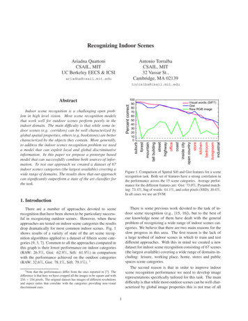
Recognizing Indoor ScenesAntonio TorralbaCSAIL, MIT32 Vassar St.,Cambridge, MA 02139Ariadna QuattoniCSAIL, MITUC Berkeley EECS & henstorecoastinside cityofficestreethighwaytall buildingforestmountainsuburbIndoor scene recognition is a challenging open problem in high level vision. Most scene recognition modelsthat work well for outdoor scenes perform poorly in theindoor domain. The main difficulty is that while some indoor scenes (e.g. corridors) can be well characterized byglobal spatial properties, others (e.g, bookstores) are bettercharacterized by the objects they contain. More generally,to address the indoor scenes recognition problem we needa model that can exploit local and global discriminativeinformation. In this paper we propose a prototype basedmodel that can successfully combine both sources of information. To test our approach we created a dataset of 67indoor scenes categories (the largest available) covering awide range of domains. The results show that our approachcan significantly outperform a state of the art classifier forthe task.open countryVisual words (SIFT)GistRaw RGB imagePercent correctAbstractFigure 1. Comparison of Spatial Sift and Gist features for a scenerecognition task. Both set of features have a strong correlation inthe performance across the 15 scene categories. Average performance for the different features are: Gist: 73.0%, Pyramid matching: 73.4%, bag of words: 64.1%, and color pixels (SSD): 30.6%.In all cases we use an SVM.1. IntroductionThere is some previous work devoted to the task of indoor scene recognition (e.g., [15, 16]), but to the best ofour knowledge none of them have dealt with the generalproblem of recognizing a wide range of indoor scenes categories. We believe that there are two main reasons for theslow progress in this area. The first reason is the lack ofa large testbed of indoor scenes in which to train and testdifferent approaches. With this in mind we created a newdataset for indoor scene recognition consisting of 67 scenes(the largest available) covering a wide range of domains including: leisure, working place, home, stores and publicspaces scene categories.The second reason is that in order to improve indoorscene recognition performance we need to develop imagerepresentations specifically tailored for this task. The maindifficulty is that while most outdoor scenes can be well characterized by global image properties this is not true of allThere are a number of approaches devoted to scenerecognition that have been shown to be particulary successful in recognizing outdoor scenes. However, when theseapproaches are tested on indoor scene categories the resultsdrop dramatically for most common indoor scenes. Fig. 1shows results of a variety of state of the art scene recognition algorithms applied to a dataset of fifteen scene categories [9, 3, 7]. Common to all the approaches compared inthis graph is their lower performance on indoor categories(RAW: 26.5%, Gist: 62.9%, Sift: 61.9%) in comparisonwith the performance achieved on the outdoor categories(RAW: 32.6%, Gist: 78.1%, Sift: 79.1%). 11 Note that the performances differ from the ones reported in [7]. Thedifference is that here we have cropped all the images to be square and with256 256 pixels. The original dataset has images of different resolutionsand aspect ratios that correlate with the categories providing non-visualdiscriminant cues.1
StoreHomebakerygrocery store clothing storedelilaundromat jewellery shopbedroomnurserychildren roomlobbyPublic spacesclosetpantryprison celllibrarywaiting roommuseumpool insideinside buscloisterLeisurechurchbuffetelevatordining room corridorrestaurantfastfoodWorking placeconcert hallbarmovie theaterhospital room kinder garden restaurant kitchen artstudioclassroomlaboratory wet studio music operating roomsubwaybookstorevideo storefloristlivingroombathroomkitchencasinoinside subwayofficegameroomcomputer roomwarehousegreen housebowlingshoe shopmalltoystorestairscasewinecellargaragelocker roomtrainstation airport insidegymhair salondental officetv studiomeeting roomFigure 2. Summary of the 67 indoor scene categories used in our study. To facilitate seeing the variety of different scene categoriesconsidered here we have organized them into 5 big scene groups. The database contains 15620 images. All images have a minimumresolution of 200 pixels in the smallest axis.indoor scenes. Some indoor scenes (e.g. corridors) can indeed be characterized by global spatial properties but others(e.g bookstores) are better characterized by the objects theycontain. For most indoor scenes there is a wide range ofboth local and global discriminative information that needsto be leveraged to solve the recognition task.In this paper we propose a scene recognition modelspecifically tailored to the task of indoor scene recognition.The main idea is to use image prototypes to define a mapping between images and scene labels that can capture thefact that images containing similar objects must have similar scene labels and that some objects are more importantthan others in defining a scene’s identity.Our work is related to work on learning distance functions [4, 6, 8] for visual recognition. Both methods learnto combine local or elementary distance functions. The aretwo main differences between their approach an ours. First,their method learns a weighted combination of elementarydistance functions for each training sample by minimizinga ranking objective function. Differently, our method learnsa weighted combination of elementary distance functionsfor a set of prototypes by directly minimizing a classification objective. Second, while they concentrated on objectrecognition and image retrieval our focus is indoor scenerecognition.This paper makes two contributions, first we provide aunique large and diverse database for indoor scene recognition. This database consists of 67 indoor categories covering a wide range of domains. Second, we introduce amodel for indoor scene recognition that learns scene prototypes similar to start-constellation models and that can successfully combine local and global image information.2. Indoor databaseIn this section we describe the dataset of indoor scenecategories. Most current papers on scene recognition focuson a reduced set of indoor and outdoor categories. In con-trast, our dataset contains a large number of indoor scenecategories. The images in the dataset were collected fromdifferent sources: online image search tools (Google andAltavista), online photo sharing sites (Flickr) and the LabelMe dataset. Fig. 2 shows the 67 scene categories used inthis study. The database contains 15620 images. All imageshave a minimum resolution of 200 pixels in the smallestaxis.This dataset poses a challenging classification problem.As an illustration of the in-class variability in the dataset,fig. 3 shows average images for some indoor classes. Notethat these averages have very few distinctive attributes incomparison with average images for the fifteen scene categories dataset and Caltech 101 [10]. These averages suggestthat indoor scene classification might be a hard task.3. Scene prototypes and ROIsWe will start by describing our scene model and the set offeatures used in the rest of the paper to compute similaritiesbetween two scenes.3.1. Prototypes and ROIAs discussed in the previous section, indoor scene categories exhibit large amounts of in-class appearance variability. Our goal will be to find a set of prototypes that bestdescribes each class. This notion of scene prototypes hasbeen used in previous works [11, 17].In this paper, each scene prototype will be defined by amodel similar to a constellation model. The main differencewith an object model is that the root node is not allowed tomove. The parts (regions of interest, ROI) are allowed tomove on a small window and their displacements are independent of each other. Each prototype Tk (with k 1.p)will be composed of mk ROIs that we will denote by tkj .Fig.4 shows an example of a prototype and a set of candidate ROIs.
bakerybarbathroombedroom60 pixels80 pixelsbookstorebuffetcasinoconcert halla) Prototype andcandidate ROIdining roomdelikitchenrestaurantpool insidemovie theaterinside busgreenhousecorridorcomputer roomairport insidemeeting roomFigure 3. Average images for a sample of the indoor scene categories. Most images within each category average to a uniformfield due to the large variability within each scene category (thisis in contrast with Caltech 101 or the 15 scene categories dataset[9, 3, 7]. The bottom 8 averages correspond to the few categoriesthat have more regularity among examplars.In order to define a set of candidate ROIs for a given prototype, we asked a human annotator to segment the objectscontained in it. Annotators segmented prototype images foreach scene category resulting in a total of 2000 manuallysegmented images. We used those segmentations to proposea set of candidate ROIs (we selected 10 for each prototypethat occupy at least 1% of the image size).We will also show results where instead of using humanannotators to generate the candidate ROIs, we used a segmentation algorithm. In particular, we produce candidateROIs from a segmentation obtained using graph-cuts [13].3.2. Image descriptorsIn order to describe the prototypes and the ROIs we willuse two sets of features that represent the state of the art onthe task of scene recognition.We will have one descriptor that will represent the rootnode of the prototype image (Tk ) globally. For this we willuse the Gist descriptor using the code available online [9].This results in a vector of 384 dimensions describing theentire image. Comparison between two Gist descriptors iscomputed using Euclidean distance.b) ROI descriptorsc) Search regionFigure 4. Example of a scene prototype. a) Scene prototype withcandidate ROI. b) Illustration of the visual words and the regionsused to compute histograms. c) Search window to detect the ROIin a new image.To represent each ROI we will use a spatial pyramid ofvisual words. The visual words are obtained as in [14]:we create vector quantized Sift descriptors by applying Kmeans to a random subset of images (following [7] we used200 clusters, i.e. visual words). Fig. 4.b shows the visualwords (the color of each pixel represents the visual wordto which it was assigned). Each ROI is decomposed into a2x2 grid and histograms of visual words are computed foreach window [7, 1, 12]. Distances between two regions arecomputed using histogram intersection as in [7].Histograms of visual words can be computed efficientlyusing integral images, this results in an algorithm whosecomputational cost is independent of window size. The detection a ROI on a new image is performed by searchingaround a small spatial window and also across a few scalechanges (Fig. 4.c). We assume that if two images are similar their respective ROIs will be roughly aligned (i.e. insimilar spatial locations). Therefore, we only need to perform the search around a small window relative to the original location. Fig. 5 shows three ROIs and its detections onnew images. For each ROI, the figure shows best and worstmatches in the dataset. The figure illustrates the variety ofROIs that we will consider: some correspond to well defined objects (e.g., bed, lamp), regions (e.g., floor, wall withpaintings) or less distinctive local features (e.g., a column,a floor tile). The next section will describe the learning algorithm used to select the most informative prototypes andROIs for each scene category.4. Model4.1. Model FormulationIn scene classification our goal is to learn a mappingfrom images x to scene labels y. For simplicity, in this section we assume a binary classification setting. That is, eachyi {1, 1} is a binary label indicating whether an imagebelongs to a given scene category or not. To model the multiclass case we use the standard approach of training oneversus-all classifiers for each scene; at test, we predict the
TargetBest matchesWorstFigure 5. Example of detection of similar image patches. The topthree images correspond to the query patterns. For each image, thealgorithm tries to detect the selected region on the query image.The next three rows show the top three matches for each region.The last row shows the three worst matching regions.scene label for which the corresponding classifier is mostconfident. However, we would like to note that our modelcan be easily adapted to an explicit multiclass training strategy.As a form of supervision we are given a training setD {(x1 , y1 ), (x2 , y2 ) . . . (xn , yn )} of n pairs of labeledimages and a set S {T1 , T2 . . . , Tp } of p segmentedimages which we call prototypes. Each prototype Tk {t1 , t2 , . . . , tmk } has been segmented into mk ROIs by ahuman annotator. Each ROI corresponds to some object inthe scene, but we do not know their labels. Our goal is touse D and S to learn a mapping h : X R. For binaryclassification, we would take the prediction of an image x tobe sign(h(x)); in the multiclass setting, we will use directlyh(x) to compare it against other class predictions.As in most supervised learning settings choosing an appropriate mapping h : X R becomes critical. In partic-ular, for the scene classification problem we would like tolearn a mapping that can capture the fact that images containing similar objects must have similar scene labels andthat some objects are more important than others in defining a scene’s identity. For example, we would like to learnthat an image of a library must contain books and shelvesbut might or might not contain tables.In order to define a useful mapping that can capture theessence of a scene we are going to use S. More specifically,for each prototype Tk we define a set of features functions:fkj (x) min d(tkj , xs )s(1)Each of these features represents the distance between aprototype ROI tkj and its most similar segment in x (seesection 3 for more details of how these features are computed). For some scene categories global image informationcan be very important, for this reason we will also include aglobal feature gk (x) which is computed as the L2 norm between the Gist representation of image x and the Gist representation of prototype k. We can then combine all thesefeature functions to define a global mapping:h(x) pXβk exp Pmkj 1λkj fkj (x) λkG gk (x)(2)k 1In the above formulation β and λ are the two parameter sets of our model. Intuitively, each βk represents howrelevant the similarity to a prototype k is for predicting thescene label. Similarly, each λkj captures the importance ofa particular ROI inside a given prototype. We can now usethe mapping h to define the standard regularized classification objective:L(β, λ) nXl(h(xi ), yi ) Cb β 2 Cl λ 2(3)i 1The left term of equation 3 measures the error that theclassifier incurs on training examples D in terms of a lossfunction l. In this paper we use the hinge loss, given byl(h(x), y) max(0, 1 yh(x)) but other losses such aslogistic loss could be used instead. The right hand termsof Equation 3 are regularization terms and the constants Cband Cl dictate the amount of regularization in the model.Finally, we introduce non-negativity constraints on the λ.Since each fkj is a distance between image ROIs, these constraints ensure that their linear combination is also a globaldistance between a prototype and an image. This eases theinterpretability of the results. Note that this global distanceis used to induce a similarity measure in the classifier h.
30%In this section we describe how to estimate the model parameters {β , λ } argminβ,λ 0 L(β, λ) from a trainingset D. The result of the learning stage will be the selectionof the relevant prototypes for each class and the ROI thatshould be used for each prototype.We use an alternating optimization strategy, which consists of a series of iterations that optimize one set of parameters given fixed values for the others. Initially the parameters are set to random values, and the process iteratesbetween fixing β and minimizing L with respect to λ andfixing λ and minimizing L with respect to β.We use a gradient-based method for each optimizationstep. Since our objective is non-differentiable because ofthe hinge loss, we use a sub-gradient of the objective, whichwe compute as follows:Given parameter values, let be the set of indices ofexamples in D that attain non-zero loss. Also, to simplifynotation assume that parameter λk0 and feature fk0 correspond to λkG and gk respectively. The subgradient withrespect to β is given by:X L yi exp βkPmkj 1λkj fkj (xi )i 1 Cb βk2and the subgradient with respect to λ is given by:X L yi βk fkj (xi ) exp λkji Pmkj 1λkj fkj (xi )1 Cl λkj2To enforce the non-negativity constraints on the λ wecombine sub-gradient steps with projections to the positiveoctant. In practice we observed that this is a simple andefficient method to solve the constrained optimization step.5. ExperimentsIn this section we present experiments for indoor scenerecognition performed on the dataset described in section2. We show that the model and representation proposedin this paper give significant improvement over a state ofthe art model for this task. We also perform experimentsusing different versions of our model and compare manualsegmentations to segmentations obtained by running a segmentation algorithm.In all cases the performance metric is the standard average multiclass prediction accuracy. This is calculated asthe mean over the diagonal values of the confusion matrix.An advantage of this metric with respect to plain multiclassaccuracy is that it is less sensitive to unbalanced distributions of classes. For all experiments we trained a one versusall classifier for each of the 67 scenes and combined theirAverage Precision4.2. Learning25%20%15%Gist SVMROISegmentationROIAnnotationROI GistSegmentationROI GistAnnotationFigure 6. Multiclass average precision performance for the baseline and four different versions of our model.scores into a single prediction by taking the scene label withmaximum confidence score. Other approaches are possiblefor combining the predictions of the different classifiers.We start by describing the four different variations of ourmodel that were tested on these experiments. In a first setting we used the ROIs obtained from the manually annotated images and restricted the model to use local information only by removing the gk (x) features (ROI Annotation).In a a second setting we allowed the model to use both local and global features (ROI Gist Annotation). In a thirdsetting we utilized the ROIs obtained by running a segmentation algorithm and restricted the model to use local information only (ROI Segmentation). Finally, in the fourthsetting we used the ROIs obtained from the automatic segmentation but allowed the model to exploit both local andglobal features (ROI Gist Segmentation). All these modelswere trained with 331 prototypes.We also compared our approach with a state of the artmodel for this task. For this we trained an SVM with a Gistrepresentation and an RBF kernel (Gist SVM). In principleother features could have been used for this baseline but asit was shown in Fig. 1 Gist is one of the most competitiverepresentations for this task.To train all the models we used 80 images of each classfor training and 20 images for testing. To train a one versusall classifier for category d we sample n positive examplesand 3n negative examples.6. ResultsFigure 6 shows the average multiclass accuracy for thefive models: Gist SVM, ROI Segmentation, ROI Annotation, ROI Gist Segmentation and ROI Gist Annotation.As we can see from this figure combining local andglobal information leads to better performance. This suggests that both local and global information are useful forthe indoor scene recognition task. Notice also that usingautomatic segmentations instead of manual segmentations
church inside 63.2%elevator 61.9%auditorium 55.6%buffet 55.0%classroom 50.0%greenhouse 50.0%bowling 45.0%cloister 45.0%concert hall 45.0%computerroom 44.4%dentaloffice 42.9%library 40.0%inside bus 39.1%closet 38.9%corridor 38.1%grocerystore 38.1%locker room 38.1%florist 36.8%studiomusic 36.8%hospitalroom 35.0%nursery 35.0%trainstation 35.0%bathroom 33.3%laundromat 31.8%stairscase 30.0%garage 27.8%gym 27.8%tv studio 27.8%videostore 27.3%gameroom 25.0%pantry 25.0%poolinside 25.0%inside subway 23.8%kitchen 23.8%winecellar 23.8%fastfood restaurant 23.5%bar 22.2%clothingstore 22.2%casino 21.1%deli 21.1%bookstore 20.0%waitingroom 19.0%dining room 16.7%bakery 15.8%livingroom 15.0%movietheater 15.0%bedroom 14.3%toystore 13.6%operating room 10.5%airport inside 10.0%artstudio 10.0%lobby 10.0%prison cell 10.0%hairsalon 9.5%subway 9.5%warehouse 9.5%meeting room 9.1%children room 5.6%shoeshop 5.3%kindergarden 5.0%restaurant 5.0%museum 4.3%restaurant kitchen 4.3%jewelleryshop 0.0%laboratorywet 0.0%mall 0.0%office 0.0%Figure 7. The 67 indoor categories sorted by multiclass averageprecision (training with 80 images per class and test is done on 20images per class).causes only a small drop in performance.Figure 7 shows the sorted accuracies for each class forthe ROI Gist-Segmentation model. Interestingly, five of thecategories (greenhouse, computer-room, inside-bus, corridor and pool-inside) for which we observed some globalregularity (see 3) are ranked among the top half best performing categories. But among this top half we also findfour categories (buffet, bathroom, concert hall, kitchen) forwhich we observed no global regularity. Figure 8 showsranked images for a random subset of scene categories forthe ROI Gist Segmentation model.Figure 9 shows the top and bottom prototypes selectedfor a subset of the categories. We can see from these resultsthat the model leverages both global and local informationat different scales.One question that we might ask is: how is the performance of the proposed model affected by the number ofprototypes used? To answer this question we tested the performance of a version of our model that used global information only for different number of prototypes (1 to 200).We observed a logarithmic growth of the average precisionas a function of the number of prototypes. This means thatby allowing the model to exploit more prototypes we mightbe able to further improve the performance.In summary, we have shown the importance of combining both local and global image information for indoorscene recognition. The model that we proposed leveragesboth and it can outperform a state of the art classifier fortask. In addition, our results let us conclude that using automatic segmentations is similar to using manual segmentations and thus our model can be trained with a minimumamount of supervision.7. ConclusionWe have shown that the algorithms that constitute theactual state of the art algorithms on the 15 scene categorization task [9, 3, 7] perform very poorly at the indoor recognition task. Indoor scene categorization represents a verychallenging task due to the large variability across different exemplars within each class. This is not the case withmany outdoor scene categories (e.g., beach, street, plaza,parking lot, field, etc.) which are easier to discriminate andseveral image descriptors have been shown to perform verywell at that task. Outdoor scene recognition, despite beinga challenging task has reached a degree of maturity that hasallowed the emergence of several applications in computervision (e.g. [16]) and computer graphics (e.g. [5]). However, most of those works have avoided dealing with indoorscenes as performances generally drop dramatically.The goal of this paper is to attract attention to the computer vision community working on scene recognition tothis important class of scenes for which current algorithmsseem to perform poorly. In this paper we have proposeda representation able to outperform representations that arethe current state of the art on scene categorization. However, the performances presented in this paper are close tothe performance of the first attempts on Caltech 101 [2].AcknowledgmentFunding for this research was provided by National Science Foundation Career award (IIS 0747120).References[1] A. Bosch, A. Zisserman, and X. Munoz. Image classificationusing rois and multiple kernel learning. Intl. J. ComputerVision, 2008.[2] L. Fei-Fei, R. Fergus, and P. Perona. Learning generativevisual models from few training examples: an incrementalbayesian approach tested on 101 object categories. In IEEE.CVPR 2004, Workshop on Generative-Model Based Vision,2004.[3] L. Fei-Fei and P. Perona. A bayesian hierarchical model forlearning natural scene categories. In cvpr, pages 524–531,2005.[4] A. Frome, Y. Singer, F. Sha, and J. Malik. Learning globallyconsistent local distance functions for shape-based imageretrieval and classification. Computer Vision, 2007. ICCV2007. IEEE 11th International Conference on, pages 1–8,Oct. 2007.[5] J. Hays and A. A. Efros. Scene completion using millions ofphotographs. ACM Transactions on Graphics, 26, 2007.[6] J. Krapac. Learning distance functions for automatic annotation of images. In Adaptive Multimedial Retrieval: Retrieval,User, and Semantics, 2008.[7] S. Lazebnik, C. Schmid, and J. Ponce. Beyond bags offeatures: Spatial pyramid matching for recognizing naturalscene categories. In cvpr, pages 2169–2178, 2006.[8] T. Malisiewicz and A. A. Efros. Recognition by associationvia learning per-exemplar distances. In CVPR, June 2008.[9] A. Oliva and A. Torralba. Modeling the shape of the scene: aholistic representation of the spatial envelope. InternationalJournal in Computer Vision, 42:145–175, 2001.
fastfood ( 0.18)garage ( 0.69)bathroom ( 0.99)kitchen ( 1.27)prisoncell ( 1.53)waitingroom ( 0.59)restaurant ( 0.89)kitchen ( 1.16)winecellar ( 1.44)classroomclassroom (2.09) classroom (1.99) classroom (1.98)pantry (1.53)fastfood ( 0.12)locker room hospitalroomdining roomrestaurant (1.57) livingroom (1.55)bathroom (2.45)bathroom (2.14)bedroom (2.01)locker room (2.52)corridor (2.27)locker room (2.22)videostore (1.44) videostore (1.39)office ( 0.04)tv studio ( 0.14)prisoncell ( 0.52) kindergarden ( 0.86) bathroom ( 1.16)bathroom ( 0.51)inside bus ( 1.37)bedroom ( 1.40)concert hall ( 0.78) concert hall ( 1.01) inside subway ( 1.22)videostoremall (1.69)laundromat (0.36) operating room( 0.23) dental office ( 0.65) bookstore ( 1.04)library (1.94)warehouse (1.93)warehouse ( 0.07) jewelleryshop ( 0.53) laundromat ( 0.87)toystore ( 1.11)bowling ( 1.32)librarylibrary (2.34)Figure 8. Classified images for a subset of scene categories for the ROI Gist Segmentation model. Each row corresponds to a scenecategory. The name on top of each image denotes the ground truth category. The number in parenthesis is the classification confidence.The first three columns correspond to the highest confidence scores. The next five columns show 5 images from the test set sampled so thatthey are at equal distance from each other in the ranking provided by the classifier. The goal is to show which images/classes are near andfar away from the decision boundary.[10] J. Ponce, T. L. Berg, M. Everingham, D. A. Forsyth,M. Hebert, S. Lazebnik, M. Marszalek, C. Schmid, B. C.Russell, A. Torralba, C. K. I. Williams, J. Zhang, and A. Zisserman. Dataset issues in object recognition. In In TowardCategory-Level Object Recognition, pages 29–48. Springer,2006.[11] A. Quattoni, M. Collins, and T. Darrell. Transfer learning forimage classification with sparse prototype representations. InCVPR, 2008.[12] B. C. Russell, A. A. Efros, J. Sivic, W. T. Freeman, andA. Zisserman. Using multiple segmentations to discover objects and their extent in image collections. In CVPR, 2006.[13] J. Shi and J. Malik. Normalized cuts and image segmentation. IEEE Transactions on Pattern Analysis and MachineIntelligence, 22(8):888–905, 1997.[14] J. Sivic and A. Zisserman. Video Google: Efficient visual search of videos. In J. Ponce, M. Hebert, C. Schmid,and A. Zisserman, editors, Toward Category-Level Object Recognition, volume 4170 of LNCS, pages 127–144.Springer, 2006.[15] M. Szummer and R. W. Picard. Indoor-outdoor image classification. In CAIVD ’98: Proceedings of the 1998 International Workshop on Content-Based Access of Image andVideo Databases (CAIVD ’98), page 42, Washington, DC,USA, 1998. IEEE Computer Society.[16] A. Torralba, K. Murphy, W. Freeman, and M. Rubin.Context-based vision system for place and object recognition. In Intl. Conf. Computer Vision, 2003.[17] A. Torralba, A. Oliva, M. S. Castelhano, and J. M. Henderson. Contextual guidance of eye movements and attention in real-world scenes: the role of global features in object search. Psychological Review, 113(4):766–786, October2006.
Beta 5.16Beta 4.85Beta 4.15Beta 3.88Beta 3.70Beta 3.30Beta 3.82Beta 3.78Beta 5.03Beta 4.99Beta 4.64Beta 4.26Beta 3.06Beta 3.00Beta 2.99Beta 3.34Beta 3.29Beta 6.73Beta 6.57Beta 6.38Beta 5.43Beta 4.75Beta 4.67Beta 4.45Beta 2.36Beta 2.04Beta 7.90Beta 5.62Beta 4.43Beta 4.42Beta 4.10Beta 4.04Beta 3.95Beta 3.46Beta 3.21Beta 3.08Beta 2.72Beta 2.54Beta 2.34Beta 2.29Beta 2.24Beta 2.13Beta 5.40Beta 4.74Beta 2.79Beta 2.60Beta 5.08BathroomBusAuditoriumChurchCasinoBeta 5.76Beta 4.53Beta 4.35Beta 3.72Beta 2.93Beta 3.93LibraryBeta 5.07Figure 9. Prototypes for a subset of scene categories and sorted by their weight. The 7 first columns correspond to the highest rankprototypes and the last two columns show prototypes with the most negative weights. The thickness of each bounding box is proportionalto the value of the weight for each ROI: λkj .
recognition that have been shown to be particulary success-ful in recognizing outdoor scenes. However, when these approaches are tested on indoor scene categories the results drop dramatically for most common indoor scenes. Fig. 1 shows results of a variety of state of the art scene recog-nition algorithms applied to a dataset of fifteen scene .