Transcription
ELECTROMAGNETICWAVE THEORY
ELECTROMAGNETICWAVE THEORYJIN AU KONGEMW PublishingCambridge, Massachusetts, USA
c 2008 by Jin Au KongCopyright Published by EMW Publishing.All rights reserved.This book is printed on acid-free paperISBN 0-9668143-9-8Manufactured in the United States of America09876543
PREFACEThis book presents a unified macroscopic theory of electromagneticwaves in accordance with the principle of special relativity from thepoint of view of the form invariance of the Maxwell equations and theconstitutive relations. Great emphasis is placed on the fundamentalimportance of the k vector in electromagnetic wave theory. We introduce a fundamental unit Ko 2π meter 1 for the spatial frequency,which is cycle per meter in spatial variation. This is similar to thefundamental unit for temporal frequency Hz, which is cycle per second in time variation. The unit Ko is directly proportional to the unitHz; one Ko in spatial frequency corresponds to 300 MHz in temporalfrequency.This is a textbook on electromagnetic wave theory, and topicsessential to the understanding of electromagnetic waves are selectedand presented. Chapter 1 presents fundamental laws and equationsfor electromagnetic theory. Chapter 2 is devoted to the treatment oftransmission line theory. Electromagnetic waves in media are studied in Chapter 3 with the kDB system developed to study wavesin anisotropic and bianisotropic media. Chapter 4 presents a detailedtreatment of reflection, transmission, guidance, and resonance of electromagnetic waves. Starting with Čerenkov radiation, we study radiation and antenna theory in Chapter 5. Chapter 6 then elaborates onthe various theorems and limiting cases of Maxwell’s theory importantto the study of electromagnetic wave behavior. Scattering by spheres,cylinders, rough surfaces, and volume inhomogeneities are treated inChapter 7. In Chapter 8, we present Maxwell’s theory from the pointof view of Lorentz covariance in accordance with the principle of special relativity. The problem section at the end of each section providesuseful exercise and applications.The various topics in the book can be taught independently, andthe material is organized in the order of increasing complexity in mathematical techniques and conceptual abstraction and sophistication.This book has been used in several undergraduate and graduate coursesthat I have been teaching at the Massachusetts Institute of Technology.–v–
viPrefaceThe first version of the book was published in 1975 by WileyInterscience, New York, entitled Theory of Electromagnetic Waves,which was based on my 1968 Ph.D. thesis, where the concept of bianisotropic media was introduced. The book was expanded and publishedin 1986 with the present title and its second edition appeared in 1990.Since 1998, it has been published by EMW Publishing Company, Massachusetts. The development of the various concepts in the book reliesheavily on published work. I have not attempted the task of referringto all relevant publications. The list of books and journal articles in theReference Section at the end of the book is at best representative andby no means exhaustive. Some of the results contained in the book aretaken from many of my research projects, which have been supportedby grants and contracts from the National Science Foundation, theNational Aeronautics and Space Administration, the Office of NavalResearch, the Army Research Office, the Jet Propulsion Laboratory ofthe California Institute of Technology, the MIT Lincoln Laboratory,the Schlumberger-Doll Research Center, the Digital Equipment Corporation, the IBM Corporation, and the funding support associatedwith the award of the S. T. Li prize for the year 2000.During the writing and preparation of the book, many peoplehelped. In particular, I would like to acknowledge Chi On Ao for formulating the TEX macros, and Zhen Wu for editing the text and constructing the index. Over the years, many of my teaching and researchassistants provided useful suggestions and proofreading, notably Leung Tsang, Michael Zuniga, Weng Chew, Tarek Habashy, Robert Shin,Shun-Lien Chuang, Jay Kyoon Lee, Apo Sezginer, Soon Yun Poh, EricYang, Michael Tsuk, Hsiu Chi Han, Yan Zhang, Henning Braunisch,Bae-Ian Wu, Xudong Chen, and Baile Zhang. I would like to expressmy gratitude to them and to the students whose enthusiastic responseand feedback continuously give me joy and satisfaction in teaching.J. A. KongCambridge, MassachusettsDecember 2007
CONTENTSChapter 1.1.11.21.31.41.51.6FUNDAMENTALS1Maxwell’s Theory3A. Maxwell’s Equations3B. Vector Analysis6Electromagnetic Waves24A. Wave Equation and Wave Solution24B. Unit for Spatial Frequency k27C. Polarization33Force, Power, and Energy45A. Lorentz Force Law45B. Lenz’ Law and Electromotive Force (EMF)53C. Poynting’s Theorem and Poynting Vector56Hertzian Waves65A. Hertzian Dipole65B. Electric and Magnetic Fields68C. Electric Field Pattern71Constitutive Relations81A. Isotropic Media82B. Anisotropic Media83C. Bianisotropic Media84D. Biisotropic Media85E. Constitutive Matrices86Boundary Conditions90A. Continuity of Electric and Magnetic FieldComponents1.790B. Surface Charge and Current Densities92C. Boundary Conditions93Reflection and Guidance98A. Wave Vector k98– vii –
viiiContentsChapter 2.2.12.22.3B. Reflection and Transmission of TE Waves99C. Reflection and Transmission of TM Waves105D. Brewster Angle and Zero Reflection107E. Guidance by Conducting Parallel Plates111Answers120TRANSMISSION LINES137Transmission Line Theory139A. Transmission Line Equations139B. Circuit Theory144Time-Domain Transmission Line Theory 153A. Wave Equations and Wave Solutions153B. Transients on Transmission Lines156C. Normal Modes and Natural Frequencies168D. Initial Value Problem170Sinusoidal Steady State TransmissionLines180A. Sinusoidal Steady State180B. Complex Impedance181C. Time Average Power186D. Generalized Reflection Coefficient187E. Normalized Complex Impedance(Smith Chart)2.4190F. Transmission Line Resonators192Lumped Element Transmission Lines201A. Lumped Element Line202B. Dispersion Relations for Lumped ElementLines2.5205C. Periodically Loaded Transmission Lines208Transmission Line Modeling215A. Modeling Reflection and Transmission215
ixChapter 3.3.13.23.3B. Modeling Antenna Radiation220C. Array Antennas225D. Array Pattern Multiplication229E. Equivalence Principle235Answers249MEDIA261Time-Harmonic Fields263A. Continuous Monochromatic Waves263B. Polarization of Monochromatic Waves265C. Time-Average Poynting Power Vector266D. Waves in Conducting Media268E. Waves in Plasma Media271F. Dispersive Media278G. Field Energy in Dispersive Media282Bianisotropic Media292A. Anisotropic Media292B. Biisotropic Media295C. Bianisotropic Media296D. Symmetry Conditions for Lossless Media297E. Reciprocity Conditions299F. Causality Relations301kDB System for Waves in Media306A. Wave Vector k306B. The kDB System309C. Maxwell Equations in kDB System313D. Waves in Isotropic Media314E. Waves in Uniaxial Media315F. Waves in Gyrotropic Media323G. Waves in Bianisotropic Media330H. Waves in Nonlinear Media339
xContentsAnswersChapter 4.4.14.2REFLECTION AND GUIDANCE353365Reflection and Transmission367A. Reflection and Transmission of TM Waves368B. Reflection and Transmission of TE Waves371C. Phase Matching373D. Total Reflection and Critical Anglel375E. Backward Waves and Negative Refraction377F. Double Refraction in Uniaxial Media378G. Total Transmission and Brewster Angle380H. Zenneck Wave382I. Plasma Surface Wave383J. Reflection and Transmission by a LayeredMedium384K. Reflection Coefficients for Stratified Media387L. Propagation Matrices and TransmissionCoefficients390Wave Guidance402A. Guidance by Conducting Parallel Plates402B. Excitation of Modes in Parallel-PlateWaveguides408C. TM Modes in Parallel-Plate Waveguides410D. Attenuation of Guided Waves Due to WallLoss411E. Guided Waves in Isotropic Medium CoatedConductor415F. Guided Waves in Layered Media422G. Guided Waves in a Symmetric SlabDielectric Waveguide425H. Cylindrical Waveguides429I. Cylindrical Rectangular Waveguides430
xi4.3Chapter 5.J. Cylindrical Circular Waveguides435Resonance462A. Rectangular Cavity Resonator462B. Circular Cavity Resonator467C. Spherical Cavity Resonator468D. Cavity Perturbation472Answers478RADIATION4875.1Čerenkov Radiation4895.2Green’s Functions495A. Dyadic Green’s Functions495B. Radiation Field Approximation499Hertzian Dipoles504A. Hertzian Electric Dipole504B. Hertzian Magnetic Dipole and Small LoopAntenna508Linear Dipole Arrays516A. Uniform Array Antenna with ProgressivePhase Shift516B. Array Antennas with Nonuniform CurrentDistributions523C. Dolph-Chebyshev Arrays526D. Array Pattern Synthesis5335.5Linear Antennas5455.6Biconical Antennas554A. Formulation and Wave Solutions554B. Solution in the Air Region and DipoleFields558C. Solution in the Antenna Region560D. Transmission Line Model5615.35.4
xiiContents5.7Chapter 6.6.1E. Formal Solution of Biconical AntennaProblem568Dipole Antennas in Layered Media572A. Integral Formulation572B. Contour Integration Methods584C. Dipole Antenna on a Two-Layer Medium607Answers633THEOREMS OF WAVES ANDMEDIA647Equivalence Principle649A. Electric and Magnetic Dipole Sources649B. Image Sources650C. Electric and Magnetic Current Sheets652D. Induced and Impressed Current Sheets654Topic 6.1A Uniqueness Theorem661Topic 6.1B Duality and Complementarity663Topic 6.1C Mathematical Formulations ofHuygens’ Principle671Topic 6.1D Fresnel and Fraunhofer Diffraction 6716.2Reaction and Reciprocity695A. Reaction695B. Reciprocity697C. Reciprocity Conditions701D. Modified Reciprocity Theorem702Topic 6.2A Stationary Formulas andRayleigh-Ritz Procedure703Topic 6.2B Method of Moments7116.3Quasi-Static Limits7156.4Geometrical Optics Limit7226.5Paraxial Limit743Topic 6.5A Gaussian Beam743
xiii6.6Chapter 7.7.17.27.37.47.57.6Quantization of Electromagnetic Waves751A. Uncertainty Principle752B. Annihilation and Creation Operators755C. Wave Quantization in Bianisotropic Media762Answers768SCATTERING771Scattering by Spheres773A. Rayleigh Scattering773B. Mie Scattering776Scattering by a Conducting Cylinder782A. Exact Solution782B. Watson Transformation784C. Creeping Waves786Scattering by Periodic Rough Surfaces789A. Scattering by Periodic CorrugatedConducting Surfaces789B. Scattering by Periodic Dielectric Surfaces793Scattering by Random Rough Surfaces801A. Kirchhoff Approximation801B. Geometrical Optics Solution811C. Small Perturbation Method815Scattering by Periodic Media825A. First-Order Coupled-Mode Equations827B. Reflection and Transmission byPeriodically-Modulated Slab829C. Far-Field Diffraction of a Gaussian Beam833D. Two-Dimensional Photonic Crystals835E. Band Gaps in One-Dimensional PeriodicalMedia837Scattering by Random Media841A. Dyadic Green’s Function for Layered Media 843
xivContents7.7Chapter 8.B. Scattering by a Half-Space RandomMedium848Effective Permittivity for a VolumeScattering Medium852A. Random Discrete Scatterers855B. Effective Permittivity for a ContinuousRandom ki Theory8758.2Lorentz Transformation879A. Lorentz Transformation of Space and Time 8798.3B. Lorentz Transformation of Field Vectors883C. Lorentz Invariants888D. Electromagnetic Field Classification890E. Transformation of Frequency and WaveVector892Topic 8.2A Aberration Effect893Topic 8.2B Doppler Effect893Waves in Moving Media903A. Transformation of Constitutive Relations903B. Waves in Moving Uniaxial Media909C. Moving Boundary Conditions913D. Phase Matching at Moving Boundaries922E. Force on a Moving Dielectric Half-Space924F. Guided Waves in a Moving Dielectric Slab927G. Guided Waves in Moving Gyrotropic Media 9298.4Maxwell Equations in Tensor Form934A. Contravariant and Covariant Vectors936B. Field Tensor and Excitation Tensor942C. Constitutive Relations in Tensor Form951
xv8.5Hamilton’s Principle and Noether’sTheorem954A. Action Integral954B. Hamilton’s Principle and MaxwellEquations955C. Noether’s Theorem and EnergyMomentum Tensors956Answers962REFERENCES969INDEX991
1FUNDAMENTALS1.1 Maxwell’s TheoryA. Maxwell’s EquationsB. Vector Analysis1.2 Electromagnetic WavesA. Wave Equation and Wave SolutionB. Unit for Spatial Frequency kC. Polarization1.3 Force, Power, and EnergyA. Lorentz Force LawB. Lenz’ Law and Electromotive Force (EMF)C. Poynting’s Theorem and Poynting Vector1.4 Hertzian WavesA. Hertzian DipoleB. Electric and Magnetic FieldsC. Electric Field Pattern1.5 Constitutive RelationsA. Isotropic MediaB. Anisotropic MediaC. Bianisotropic MediaD. Biisotropic MediaE. Constitutive Matrices–1–
21. Fundamentals1.6 Boundary ConditionsA. Continuity of Electric and Magnetic Field ComponentsB. Surface Charge and Current DensitiesC. Boundary Conditions1.7 Reflection and GuidanceA. Wave Vector kB. Reflection and Transmission of TE WavesC. Reflection and Transmission of TM WavesD. Brewster Angle and Zero ReflectionE. Guidance by Conducting Parallel PlatesAnswers
1.1 Maxwell’s Theory1.13Maxwell’s TheoryA. Maxwell’s EquationsThe laws of electricity and magnetism were established in 1873 byJames Clerk Maxwell (1831–1879). In three-dimensional vector notation, the Maxwell equations are D J t E B t H (1.1.1)(1.1.2) ·D ρ(1.1.3) ·B 0(1.1.4)where E, B, H, D, J, and ρ are real functions of position and time.E electric field strength(volts/m)B magnetic flux density(webers/m2 )H magnetic field strength(amperes/m)(coulombs/m2 )D electric displacementJ electric current density(amperes/m2 )ρ electric charge density(coulombs/m3 )Equation (1.1.1) is Ampère’s law or the generalized Ampère circuit law.Equation (1.1.2) is Faraday’s law or Faraday’s magnetic induction law.Equation (1.1.3) is Coulomb’s law or Gauss’ law for electric fields.Equation (1.1.4) is Gauss’ law or Gauss’ law for magnetic fields.We generally refer to E and D as electric fields, and H and Bas magnetic fields.Maxwell’s contribution to the laws of electricity and magnetism isthe term D/ t , which is called the displacement current. The addition of the displacement current to the electric current density J (r, t)in the original Ampère’s law has at least three major consequences.First, in a capacitor which is an open circuit for direct current, thedisplacement current insures the continuity of alternating currents inelectric circuits. Secondly, the continuity law ·J ρ t(1.1.5)
41. Fundamentalsfollows from (1.1.1) and (1.1.3) by making use of the vector identity · ( H) 0 . It is the displacement term that guarantees theconservation of electric current and charge densities. Eq. (1.1.5) statesthat the electric current and charge densities are conserved at all time.Thirdly, Faraday’s law in (1.1.2) states that surrounding a time-varyingmagnetic field, electric fields are produced, and are also time-varying.With the displacement term in (1.1.1), Ampère’s law states that aroundtime-varying electric fields, time-varying magnetic fields are produced.This interrelationship between the time-varying electric and magneticfields constitutes the foundation of electromagnetic wave theory andled Maxwell to the prediction of electromagnetic waves.In developing his theory for the electromagnetic fields in spaceand time, Maxwell conceived of a substance filling the whole spacecalled aether. In the aether, the electric fields D and E are relatedby a dielectric permittivity o , and the magnetic fields B and H arerelated by a magnetic permeability µo .D oEB µo Hwhereo 8.85 10 12µo 4π 10 7(1.1.6a)(1.1.6b)farad/meterhenry/meterwhere the numerical values for o and µo are expressed in MKS units.We now call (1.1.6) the constitutive relations for free space.With Equations (1.1.1)–(1.1.6), Maxwell’s theory of electromagnetic fields is completely expressed. Originally written in Cartesiancomponent form, Maxwell’s equations were cast in the current vectorform by Oliver Heaviside (1850–1925). In 1888, Heinrich Rudolf Hertz(1857–1894) demonstrated the generation of radio waves and experimentally verified Maxwell’s theory. Since then, electromagnetic theoryhas played a central role in the development of radio, television, wireless communications, radar, microwave heating, remote sensing, andnumerous other practical applications. The special theory of relativitydeveloped by Albert Einstein (1879–1955) in 1905 further asserted therigorousness and elegance of Maxwell’s theory. As a well-establishedscientific discipline, this sophisticated theoretical structure embodiesmany principles and concepts which serve as fundamental rules of nature and vital links for all scientific disciplines.
1.1 Maxwell’s Theory5James Clerk Maxwell (13 June 1831 – 5 November 1879)James Clerk Maxwell attended University of Edinburgh (1847–1850),and studied under William Hopkins at Cambridge University (1850–1854).He was a fellow of Trinity (1855–1856), Professor of Natural Philosophy atMarischal College of the University of Aberdeen (1856–1860), and at King’sCollege (1860–1865). He was the first Cavendish Professor of ExperimentalPhysics at Cambridge University to build and direct the Cavendish Laboratory (1871–1879). He published four books and about 100 papers starting atage 14, including ‘On Faraday’s Lines of Forces’ in 1855, ‘On Physical Linesof Force’ in 1861, and ‘A Dynamical Theory of the Electromagnetic Field’ in1864. In 1865, at age 33, he retired to his country home estate to write hismonumental book A Treatise of Electricity and Magnetism (Constable andCompany, London, 1873; Dover Publications, New York, 1006 pages, 1954).Michael Faraday (22 September 1791 – 25 August 1867)Faraday became an assistant to Sir Humphry Davy at the Royal Institution on 1 March 1813. In September 1821, his experimentation demonstratedelectro-magnetic rotation, initiated the concept of electric motor. In August1831, he discovered electro-magnetic induction, and that magnetism producedelectricity through movement, the principle behind the electric transformerand generator. He became professor of chemistry in 1833. Faraday publishedmany of his results in the three-volume Experimental Researches in Electricity(1839–1855).Johann Carl Friedrich Gauss (30 April 1777 – 23 February 1855)Gauss studied mathematics at the University of Göttingen from 1795 to1798, and received his doctoral degree from the University of Helmstedt in1799. In 1807 he took the position of director of the Göttingen Observatory.In 1832 he presented a systematic use of absolute units (length, mass, time)to measure nonmechanical quantities. From 1831 to 1837 he worked closelywith Wilhelm Eduard Weber (24 October 1804 – 23 June 1891) on terrestrialmagnetism and organized a system of stations for systematic observations.André-Marie Ampère (20 January 1775 – 10 June 1836)Ampère was appointed professor at Bourg Ecole Centrale in 1802, atthe Ecole Polytechnique in 1809, and at Université de France in 1826. InSeptember 1820, Ampère showed that two parallel conductors attract eachother if they carry currents that flow in the same direction and repel if thecurrents flow in opposite directions. In 1823–1826, he completed his memoir onthe ‘Mathematical Theory of Electrodynamic Phenomena, Uniquely Deducedfrom Experience’.Charles-Augustin de Coulomb (14 June 1736 – 23 August 1806)Coulomb worked in the Corps du Génie until he retired in 1791. In 1777he invented the torsion balance, which enabled him to establish the fundamental laws of electricity by measuring the force between two small spherescharged with electricity. Between 1785 and 1791, he published seven treatiseson electricity and magnetism.
61. FundamentalsB. Vector AnalysisA vector A has a magnitude and a direction, which can be representedgraphically by a straight-line element of length proportional to themagnitude of A and with an arrow pointing in the direction of A . Ina Cartesian coordinate system (also called the rectangular coordinatesystem), we write in terms of the three Cartesian components Ax , Ay ,and Az [Fig. 1.1.1].zAzAẑŷAyx̂yAxxFigure 1.1.1 Projection of A in rectangular coordinate system.A x̂Ax ŷAy ẑAzwhere Ax , Ay , Az are the projections of A onto the x, y, z axes. Wedenote the directions of the x, y, z axes with x̂, ŷ, ẑ each of themhas unit magnitude with the scalar product x̂ · x̂ ŷ · ŷ ẑ · ẑ 1 .They are called the unit vectors. Furthermore x̂ · ŷ ŷ · ẑ ẑ · x̂ 0 .We use a hat instead of an overbar to represent the vector with unitmagnitude.Rene Descartes (31 March 1596 – 11 February 1650)Rene Descartes originated the Cartesian coordinates and founded analytic geometry. His philosophy is called Cartesianism (from Cartesius, theLatin form of his name), with the famous statement ‘I think, therefore I am.’He preached universal doubt; only one thing cannot be doubted: doubt itself.
1.1 Maxwell’s Theory7Vector Addition and SubtractionTwo vectors A and B , when they are not in the same direction or inopposite directions, determine a plane. In Cartesian components, we writeA x̂Ax ŷAy ẑAzB x̂Bx ŷBy ẑBzIt follows thatA B x̂(Ax Bx ) ŷ(Ay By ) ẑ(Az Bz )Scalar Dot ProductThe scalar or dot product of two vectors A and B , denoted by A · B ,is a scalar number,A · B Ax Bx Ay By Az BzVector Cross ProductThe vector or cross product of two vectors A and B , denoted by A B ,is a vector. In terms of their Cartesian components,A B x̂(Ay Bz Az By ) ŷ(Az Bx Ax Bz ) ẑ(Ax By Ay Bx ) x̂ŷẑ Ax A y A z B B B xyzFor the three orthogonal unit vectors x̂, ŷ, and ẑ it is seen that x̂ ŷ ẑ, ŷ ẑ x̂, ẑ x̂ ŷ.The direction of A B follows the right-hand rule, i.e., when the fingersof the right hand rotate from A to B , the thumb of the right hand points inthe direction of A B . Thus the vector A B is perpendicular to both Aand B and the plane containing A and B . It is seen that for A x̂Ax ŷAyand B x̂Bx ŷBy both in the xy -plane, A B ẑ(Ax By Ay Bx ) is inthe ẑ direction perpendicular to both A and B .Division by a vector is not defined; thus B/A and 1/A are meaninglessexpressions. If none of the operations of addition, subtraction, dot product,or cross product is imposed on A and B , the entity A B is called a dyad.In the language of tensor analysis, a dyad is a tensor of second rank, whileall vectors are tensors of first rank.
81. FundamentalsOperation of Three VectorsFor three vectors A , B , and C , we haveC · (A B) A · (B C) B · (C A)(1.1.7) Cx Cy Cz Ax Ay Az Bx By Bz Ax Ay Az Bx By Bz Cx Cy Cz B B B C C C A A A xyzxyzxyzC (A B) x̂ [Cy (Ax By Ay Bx ) Cz (Az Bx Ax Bz )] ŷ [Cz (Ay Bz Az By ) Cx (Ax By Az By )] ẑ [Cx (Az Bx Ax Bz ) Cy (Ax By Ay Bx )] (x̂Ax ŷAy ẑAz )(Cx Bx Cy By Cz Bz ) (Cx Ax Cy Ay Cz Az )(x̂Bx ŷBy ẑBz ) A(C · B) (C · A)B(1.1.8)Notice that the vector C (A B) is perpendicular to C and lies in theplane determined by A and B .Operation with the del OperatorThe del operator is a vector differential operator written as x̂ ŷ ẑ x y zThe following can be proved in Cartesian coordinates or in vector form: · (E H) H · ( E) E · ( H)(1.1.9) · ( A) 0(1.1.10) ( Φ) 0(1.1.11) ( E) ( · E) 2 E(1.1.12)where 2 · 2 2 2 x2 y 2 z 2(1.1.13)is the Laplacian operator in the rectangular coordinate system.Pierre-Simon Laplace (28 March 1749 – 5 March 1827)Pierre-Simon Laplace was appointed to a chair of mathematics at theÉcole Militaire in Paris at the age of 19. During the French Revolution hehelped to establish the metric system. The Laplace equation 2 · Φ 0 waspublished in 1813.
1.1 Maxwell’s Theory9Gradient of a ScalarWhen the del operator operates on a scalar function Φ(x, y, z), the result is a vector Φ x̂ Φ ŷ Φ ẑ Φ x y z(1.1.14)called the gradient of Φ(x, y, z). The differential form of the gradient of Φ as definedstates that Φ Φ Φ ŷ lim ẑ lim y 0 y z 0 z x·µ¶ x1 xΦ(x , y, z) Φ(x , y, z) x̂ lim x 0 x22·µ¶ 1 y yΦ(x, y , z) Φ(x, y , z) ŷ lim y 0 y22·µ¶ 1 z zΦ(x, y, z ) Φ(x, y, z ) ẑ lim z 0 z22 Φ x̂ lim x 0(1.1.15)When Φ(x, y, z) Φ(x) is a function of x only, Φ(x) is a vector pointing in thedirection of increasing x with the magnitude equal to the slope of the function atx.EXAMPLE 1.1.1 Electric field vector as gradient of a potential function.When there is no time variation, we may write the electric field vector E asE Φ(E1.1.1.1)and call Φ a potential function. As the gradient Φ points in the direction ofincreasing potential Φ, the electric field E points from high potential towards lowpotential, similar to water flowing from a high altitude to lower ground.Giving the potential of a point charge Q isΦ Q4πrthe electric field is QΦ r4πr2Thus the electric field points from high potential to low potential.E —END OF EXAMPLE 1.1.1—
101. FundamentalsDivergence of a VectorThe divergence of a vector function is a scalar, defined as · D x̂· (x̂Dx ŷDy ẑDz ) ŷ ẑ x y z Dx Dy Dz x y z(1.1.16)z(x0 , y0 , z0 ) z x yyxFigure 1.1.2 Differential volume x y z .Consider a differential volume with sides x, y, z centered around apoint (x0 , y0 , z0 ) [Fig. 1.1.2]. The divergence as defined states that 1 x x ·D lim y z Dx (x0 , y0 , z0 ) Dx (x0 , y0 , z0 ) x 0 x y z22 y 0 z 0 y y z x Dy (x0 , y0 , z0 ) Dy (x0 , y0 , z0 )zz z z) Dz (x0 , y0 , z0 ) x y Dz (x0 , y0 , z0 22(1.1.17)
1.1 Maxwell’s Theory11Gauss Theorem or Divergence TheoremThe first term in the braces is equal to the field component Dx at thesurface at x x0 x2 multiplied by the surface area y z . We define asurface normal vector dS pointing outward of the volume such that at the xsurface at x x0 x2 , dS x̂ y z and at the surface at x x0 2 ,dS x̂ y z . Then the negative sign in the second term is due to D dotmultiplied by dS . All six terms account for the six differential areas boundingthe differential volume V x y z with a surface normal dS . We thusexpress the divergence of D as · D lim V 01 dS · D V(1.1.18)Applying (1.1.18) to a large volume V containing an infinite number of suchinfinitesimal differential volumes [Fig. 1.1.3], we note that integrating the divergence over the volume surfaces shared by adjacent differential volumes willhave no contribution because the surface normals point in opposite directionsand thus cancel. The result is the divergence theorem or Gauss theoremVSFigure 1.1.3 Derivation of divergence theorem.dV · D dS · DV(1.1.19)SThe divergence theorem states that the volume integral of the divergence ofthe vector field D is equal to the total outward flux D through the surfaceS enclosing the volume.
121. FundamentalsCurl of a VectorThe curl of a vector field H is a vector defined as H x̂ x̂ ŷ ẑ x y z Hz Hy ŷ y z H x̂ xHxŷ yHy Hx Hz ẑ z x ẑ z Hz Hy Hx x y (1.1.20)Consider a differential volume of sides x, y, z centered around a point(x0 , y0 , z0 ) . In the Cartesian coordinate system, the differential form of thecurl of H as defined states that H lim x 0 y 0 z 0 1x̂ x 1 ŷ y x xH(x0 , y0 , z0 ) H(x0 , y0 , z0 )22 y y, z0 ) H(x0 , y0 , z0 )H(x0 , y0 22 1 z z) H(x0 , y0 , z0 ) ẑ H(x0 , y0 , z0 z221 lim x 0 x y z y 0 z 0 x̂ x z x y y z z zHx (x0 , y0 , z0 ) Hx (x0 , y0 , z0 )22 x x, y0 , z0 ) Hz (x0 , y0 , z0 )Hz (x0 22 ẑ y z x z z zHy (x0 , y0 , z0 ) Hy (x0 , y0 , z0 )22 ŷ x y y yHz (x0 , y0 , z0 ) Hz (x0 , y0 , z0 )22 x xHy (x0 , y0 , z0 ) Hy (x0 , y0 , z0 )22 y yHx (x0 , y0 , z0 ) Hx (x0 , y0 , z0 )22(1.1.21)
1.1 Maxwell’s Theory13Stokes TheoremThe ẑ component of (1.1.21) is Hy Hx x y 1 x x lim y Hy (x0 , y0 , z0 ) Hy (x0 , y0 , z0 ) x 0 x y22 y 0ẑ · ( H) ( H)z y y x Hx (x0 , y0 , z0 ) Hx (x0 , y0 , z0 )22The first term in the bracket is equal to the component Hy at x x0 x2multiplied by the differential length y . We define a vector differential lengthdl [Fig. 1.1.4] such that for the side y at x x0 x2 , dl ŷdy ; for ythe side x at y0 2 , dl x̂dx ; for the side y at x x0 x2 ,dl ŷdy ; and for the side x at y y0 y,dl x̂dx.Ifweuse2the fingers of the right hand to trace the direction of dl along the loop, theright-hand thumb points in the surface normal direction ẑ . Thusẑ y(x0 , y0 )dl x̂dxdl ŷdyC xFigure 1.1.4 Derivation of ẑ -component of the curl of a vector field.ẑ · ( H) lim x 0 y 01 Sdl · H(1.1.22)Cwhere C denotes the contour circulating the area S x y . Similarresults are derivable for the x̂ and ŷ components of H . For a differentialarea S with a surface normal in the direction of ŝ , we haveŝ · ( H) lim S 01 Sdl · HC(1.1.23)
141. FundamentalsWe now apply (1.1.21) to an open surface S , subdivide into N differentialareas [Fig. 1.1.5]. For a differential area Sj bounded by a contour Cj andwith a surface normal sˆj , we have S j sˆj Sj and S j · ( H)j dl · HCjAdding the contributions of all N differential areas [Fig. 1.1.5], we findNlim Sj 0N j 1 S j · ( H)j dl · HC SCCSCFigure 1.1.5 Derivation of Stokes’ theorem.Since the common part of the contours in two adjacent elements is traversedin opposite directions by the two contours, the net contribution of all thecommon parts in the interior sums to zero and only the contribution from theexternal contour C bounding the open surface S remains in the line integralon the right-hand side. The left-hand side becomes a surface integral, and theresult is Stokes’ theorem:dS · ( H) dl · H(1.1.24)CStokes’ theorem states that the surface integral of the curl of the vector fieldH over an open surface S is equal to the closed line integral of the vectoralong the contour enclosing
The first version of the book was published in 1975 by Wiley Interscience, New York, entitled Theory of Electromagnetic Waves, which was based on my 1968 Ph.D. thesis, where the concept of bian-isotropic media was introduced. The book was expanded and published in 1986 with the present title and its second edition appeared in 1990.