WIXLIB

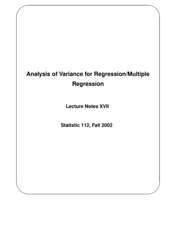
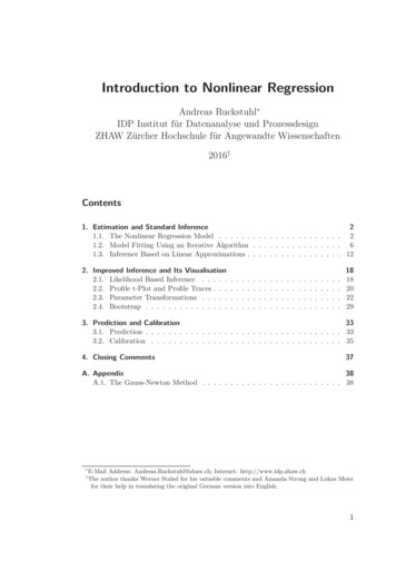
Nonparametric Regression Analysis21Nonparametric Regression Analysis22Infant Mortality Rate per 100050100150Treating a discrete quantitative predictor variable as a set of categoriesand binning continuous predictor variables are common strategies in theanalysis of large datasets. Often continuous variables are implicitly binned in the process of datacollection, as in a sample survey that asks respondents to report incomein class intervals (e.g., 0– 5000, 5000– 10,000, 10,000– 15,000,etc.). If there are sufficient data to produce precise estimates, then usingdummy variables for the values of a discrete predictor or for the classintervals of a binned predictor is preferable to blindly assuming linearity.0 An even better solution is to compare the linear and nonlinear specifications.010000200003000040000GNP Per Capita, U.S. DollarsFigure 5. The binning estimator applied to the relationship between infantmortality and GDP per capita.c 2005 by John Fox ESRC Oxford Spring SchoolNonparametric Regression Analysis233.1.2 Statistical Considerations*The mean-squared error of estimation is the sum of squared bias andsampling variance:MSE[ fb(x0)] bias2[fb(x0)] V [ fb(x0)]As is frequently the case in statistical estimation, minimizing bias andminimizing variance work at cross purposes: Wide bins produce small variance and large bias.c 2005 by John Fox Nonparametric Regression AnalysisESRC Oxford Spring School24Even though the binning estimator is biased, it is consistent as longas the population regression function is reasonably smooth. All we need do is shrink the bin width to 0 as the sample size n grows,but shrink it sufficiently slowly that the number of observations in eachbin grows as well. Under these circumstances, bias[ fb(x)] 0 and V [ fb(x)] 0 asn . Small bins produce large variance and small bias. Only if we have a very large sample can we have our cake and eat it too. All methods of nonparametric regression bump up against this problemin one form or another.c 2005 by John Fox ESRC Oxford Spring Schoolc 2005 by John Fox ESRC Oxford Spring School

Nonparametric Regression Analysis273. Fitted values are calculated for each focal x (in this case x(1), x(2), ., x(102))and then connected, as in panel (c).c 2005 by John Fox ESRC Oxford Spring SchoolNonparametric Regression Analysis In addition to the obvious flattening of the regression curve at the leftand right, local averages can be rough, because fb(x) tends to take smalljumps as observations enter and exit the window. The kernel estimator(described shortly) produces a smoother result.28(a)(b)x(80)Prestige80x(80)20 Local averages are also subject to distortion when outliers fall in thewindow, a problem addressed by robust estimation.80ESRC Oxford Spring School2. The y -values associated with these observations are averaged,producing the fitted value yb(80) in panel (b).60c 2005 by John Fox 1. The window shown in panel (a) includes the m 40 nearest neighborsof the focal value x(80).Prestige As in binning, we can employ a window of fixed width w centered on thefocal value x0, or can adjust the width of the window to include a constantnumber of observations, m. These are the m nearest neighbors of thefocal value.Figure 6 shows how local averaging works, using the relationship ofprestige to income in the Canadian occupational prestige data.y (80)40spread within the range of observed x-values, or at the (ordered)observations, x(1), x(2), ., x(n).2620The essential idea behind local averaging is that, as long as the regressionfunction is smooth, observations with x-values near a focal x0 areinformative about f (x0). Local averaging is very much like binning, except that rather thandissecting the data into non-overlapping bins, we move a bin (called awindow) continuously over the data, averaging the observations that fallin the window. We can calculate fb(x) at a number of focal values of x, usually equallyNonparametric Regression Analysis Problems occur near the extremes of the x’s. For example, all of thenearest neighbors of x(1) are greater than or equal to x(1), and thenearest neighbors of x(2) are almost surely the same as those of x(1),producing an artificial flattening of the regression curve at the extremeleft, called boundary bias. A similar flattening occurs at the extremeright, near x(n).60253.1.3 Local Averaging40Nonparametric Regression Analysis0500010000 15000 20000 25000Income0500010000 15000 20000 25000Income604020Prestige80(c)0500010000 15000 20000 25000IncomeFigure 6.Nonparametric regression of prestige on income usinglocal averages.c 2005 by John Fox ESRC Oxford Spring Schoolc 2005 by John Fox ESRC Oxford Spring School

Nonparametric Regression Analysis293.2 Kernel Estimation (Locally Weighted Averaging)Kernel estimation is an extension of local averaging. The essential idea is that in estimating f (x0) it is desirable to give greaterweight to observations that are close to the focal x0. Let zi (xi x0)/h denote the scaled, signed distance between thex-value for the ith observation and the focal x0. The scale factor h,called the bandwidth of the kernel estimator, plays a role similar to thewindow width of a local average. We need a kernel function K(z) that attaches greatest weight to observations that are close to the focal x0, and then falls off symmetrically andsmoothly as z grows. Given these characteristics, the specific choiceof a kernel function is not critical.c 2005 by John Fox ESRC Oxford Spring SchoolNonparametric Regression Analysis31Nonparametric Regression Analysis30 Having calculated weights wi K[(xi x0)/h], we proceed to computea fitted value at x0 by weighted local averagingof the y ’s:Pnwyi ifb(x0) yb x0 Pi 1ni 1 wi Two popular choices of kernel functions, illustrated in Figure 7, are theGaussian or normal kernel and the tricube kernel:– The normal kernel is simply the standard normal density function,12KN (z) e z /22πHere, the bandwidth h is the standard deviation of a normal distributioncentered at x0.c 2005 by John Fox ESRC Oxford Spring SchoolNonparametric Regression Analysis32– The tricube kernel is½(1 z 3)3 for z 1for z 10For the tricube kernel, h is the half-width of a window centered at thefocal x0. Observations that fall outside of the window receive 0 weight.0.81.0KT (z) 0.00.2K(z)0.4 0.6– Using a rectangular kernel (also½ shown in Figure 7)1 for z 1KR(z) 0 for z 1gives equal weight to each observation in a window of half-width hcentered at x0, and therefore produces an unweighted local average.-2-1012Figure 7. Tricube (light solid line), normal (broken line, rescaled) and rectangular (heavy solid line) kernel functions.c 2005 by John Fox ESRC Oxford Spring Schoolc 2005 by John Fox ESRC Oxford Spring School

Nonparametric Regression Analysis33I have implicitly assumed that the bandwidth h is fixed, but the kernelestimator is easily adapted to nearest-neighbour bandwidths. The adaptation is simplest for kernel functions, like the tricube kernel,that fall to 0: Simply adjust h(x) so that a fixed number of observationsm are included in the window. The fraction m/n is called the span of the kernel smoother.Nonparametric Regression Analysis34Kernel estimation is illustrated in Figure 8 for the Canadian occupational prestige data. Panel (a) shows a neighborhood containing 40 observations centered onthe 80th ordered x-value. Panel (b) shows the tricube weight function defined on the window; thebandwidth h[x(80)] is selected so that the window that accommodates the40 nearest neighbors of the focal x(80). Thus, the span of the smootheris 40/102 ' .4. Panel (c) shows the locally weighted average, yb(80) yb x(80). Panel (d) connects the fitted values to obtain the kernel estimate of theregression of prestige on income. In comparison with the local-averageregression, the kernel estimate is smoother, but it still exhibits flatteningat the boundaries.c 2005 by John Fox ESRC Oxford Spring SchoolNonparametric Regression Analysis35(a)x (80)360.60.0200.20.4Tricube Weight0.88060Prestige40Nonparametric Regression AnalysisESRC Oxford Spring SchoolVarying the bandwidth of the kernel estimator controls the smoothnessof the estimated regression function: Larger bandwidths produce smootherresults. Choice of bandwidth will be discussed in more detail in connectionwith local polynomial regression.(b)1.0x(80)c 2005 by John Fox 0500010000 15000 20000 2500010000 15000 20000 25000(d)60Prestige2040y 0010000 15000 20000 25000Income0500010000 15000 20000 25000IncomeFigure 8. The kernel estimator applied to the Canadian occupational prestige data.c 2005 by John Fox ESRC Oxford Spring Schoolc 2005 by John Fox ESRC Oxford Spring School

Nonparametric Regression Analysis373.3 Local Polynomial RegressionLocal polynomial regression corrects some of the deficiencies of kernelestimation. It provides a generally adequate method of nonparametric regressionthat extends to multiple regression, additive regression, and generalizednonparametric regression.Nonparametric Regression Analysis38Perhaps you are familiar with polynomial regression, where a p-degreepolynomial in a predictor x,y α β 1x β 2x2 · · · β pxp εis fit to data, usually by the method of least squares: p 1 corresponds to a linear fit, p 2 to a quadratic fit, and so on. Fitting a constant (i.e., the mean) corresponds to p 0. An implementation of local polynomial regression called lowess (orloess) is the most commonly available method of nonparametricregression.c 2005 by John Fox ESRC Oxford Spring SchoolNonparametric Regression Analysis39Local polynomial regression extends kernel estimation to a polynomialfit at the focal point x0, using local kernel weights, wi K[(xi x0)/h].The resulting weighted least-squares (WLS) regression fits the equationyi a b1(xi x0) b2(xi x0)2 · · · bp(xi x0)p eiPto minimize the weighted residual sum of squares, ni 1 wie2i . Once the WLS solution is obtained, the fitted value at the focal x0 is justyb x0 a. As in kernel estimation, this procedure is repeated for representativefocal values of x, or at the observations xi. The bandwidth h can either be fixed or it can vary as a function of thefocal x.c 2005 by John Fox ESRC Oxford Spring SchoolNonparametric Regression Analysis40 The number of observations included in each window is then m [sn], where the square brackets denote rounding to the nearest wholenumber.Selecting p 1 produces a local linear fit, the most common case. The ‘tilt’ of the local linear fit promises reduced bias in comparison withthe kernel estimator, which corresponds to p 0. This advantage ismost apparent at the boundaries, where the kernel estimator tends toflatten. The values p 2 or p 3, local quadratic or cubic fits, produce moreflexible regressions. Greater flexibility has the potential to reduce biasfurther, but flexibility also entails the cost of greater variation. When the bandwidth defines a window of nearest neighbors, as isthe case for tricube weights, it is convenient to specify the degree ofsmoothing by the proportion of observations included in the window.This fraction s is called the span of the local-regression smoother. There is a theoretical advantage to odd-order local polynomials, so p 1is generally preferred to p 0, and p 3 to p 2.c 2005 by John Fox c 2005 by John Fox ESRC Oxford Spring SchoolESRC Oxford Spring School

Nonparametric Regression Analysis42(a)x (80)(b)0.60.4Tricube Weight0.2Prestige0.8801.0x (80)600.0200 The locally weighted linear fit appears in panel (c). Fitted values calculated at each observed x are connected in panel (d).There is no flattening of the fitted regression function, as there was forkernel estimation.500010000 15000 20000 2500010000 15000 20000 25000(d)2040y (80)Prestige6080(c)20Prestige5000Income80x (80)0Income60 Panel (b) shows the tricube weight function defined on this window.4041Figure 9 illustrates the computation of a local linear regression fit tothe Canadian occupational prestige data, using the tricube kernel functionand nearest-neighbour bandwidths. Panel (a) shows a window corresponding to a span of .4, accommodatingthe [.4 102] 40 nearest neighbors of the focal value x(80).40Nonparametric Regression Analysis0500010000 15000 20000 25000Income0500010000 15000 20000 25000Average IncomeFigure 9. Nearest-neighbor local linear regression of prestige on income.c 2005 by John Fox ESRC Oxford Spring SchoolNonparametric Regression Analysis433.3.1 Selecting the Span by Visual Trial and ErrorI will assume nearest-neighbour bandwidths, so bandwidth choice isequivalent to selecting the span of the local-regression smoother. Forsimplicity, I will also assume a locally linear fit.c 2005 by John Fox Nonparametric Regression AnalysisESRC Oxford Spring School44An illustration, for the Canadian occupational prestige data, appearsin Figure 10. For these data, selecting s .5 or s .7 appears to providea reasonable compromise between smoothness and fidelity to the data.A generally effective approach to selecting the span is guided trial anderror. The span s .5 is often a good point of departure. If the fitted regression looks too rough, then try increasing the span; ifit looks smooth, then see if the span can be decreased without makingthe fit too rough. We want the smallest value of s that provides a smooth fit.c 2005 by John Fox ESRC Oxford Spring Schoolc 2005 by John Fox ESRC Oxford Spring School

Nonparametric Regression Analysis45Nonparametric Regression Analysis463.3.2 Selecting the Span by Cross-Validation*10000150002000025000Prestige6080A conceptually appealing, but complex, approach to bandwidth selectionis to estimate the optimal h (say h ). We either need to estimate h (x0)for each value x0 of x at which yb x is to be evaluated, or to estimate anoptimal average value to be used with the fixed-bandwidth estimator. Asimilar approach is applicable to the nearest-neighbour local-regressionestimator. The so-called plug-in estimate of h proceeds by estimating its components, which are the error variance σ 2, the curvature of the regressionfunction at the focal x0, and the density of x-values at x0. To do thisrequires a preliminary estimate of the regression s 0.7s 40Prestige6080Income40Prestige40205000800Prestiges 0.580s 0.380s 000025000IncomeFigure 10. Nearest-neighbor local linear regression of prestige on income,for several values of the span s.c 2005 by John Fox ESRC Oxford Spring SchoolNonparametric Regression Analysis47 A simpler approach is to estimate the optimal bandwidth or span bycross-validation In cross-validation, we evaluate the regression functionat the observations xi.– The key idea in cross-validation is to omit the ith observation from thelocal regression at the focal value xi. We denote the resulting estimateof E(y xi) as yb i xi. Omitting the ith observation makes the fitted valueyb i xi independent of the observed value yi.– The cross-validation functionPisCV(s) ny i(s)i 1 [b yi]2nwhere yb i(s) is yb i xi for span s. The object is to find the value of sthat minimizes CV.– In practice, we need to compute CV(s) for a range of values of s.c 2005 by John Fox ESRC Oxford Spring SchoolNonparametric Regression Analysis48– Although cross-validation is often a useful method for selectingthe span, CV(s) is only an estimate, and is therefore subject tosampling variation. Particularly in small samples, this variability canbe substantial. Moreover, the approximations to the expectation andvariance of the local-regression estimator are asymptotic, and in smallsamples CV(s) often provides values of s that are too small.– There are sophisticated generalizations of cross-validation that arebetter behaved.Figure 11 shows CV(s) for the regression of occupational prestige onincome. In this case, the cross-validation function provides little specifichelp in selecting the span, suggesting simply that s should be relativelylarge. Compare this with the value s ' .6 that we arrived at by visual trialand error.– Other than repeating the local-regression fit for different values ofs, cross-validation does not increase the burden of computation,because we typically evaluate the local regression at each xi anyway.c 2005 by John Fox ESRC Oxford Spring Schoolc 2005 by John Fox ESRC Oxford Spring School

Nonparametric Regression Analysis49Nonparametric Regression Analysis502503.4 Making Local Regression Resistant to Outliers*CV(s)200As in linear least-squares regression, outliers — and the heavy-tailederror distributions that generate them — can wreak havoc with thelocal-regression least-squares estimator. One solution is to down-weight outlying observations. In linear regression, this strategy leads to M -estimation, a kind of robust regression.150 The same strategy is applicable to local polynomial regression.100Suppose that we fit a local regression to the data, obtaining estimatesybi and residuals ei yi ybi. Large residuals represent observations that are relatively remote fromthe fitted regression.0.00.20.40.60.81.0Figure 11. Cross-validation function for the local linear regression of prestige on income.c 2005 by John Fox ESRC Oxford Spring SchoolNonparametric Regression Analysis51 Now define weights Wi W (ei), where the symmetric function W (·)assigns maximum weight to residuals of 0, and decreasing weight as theabsolute residuals grow.– One popular choice of weightis the bisquare or biweight: function³ e 2 2 i1 for ei cSWi WB (ei) cS for ei cS0where S is a measure of spread of the residuals, such as S median ei ; and c is a tuning constant.– Smaller values of c produce greater resistance to outliers but lowerefficiency when the errors are normally distributed.– Selecting c 7 and using the median absolute deviation producesabout 95-percent efficiency compared with least-squares when theerrors are normal; the slightly smaller value c 6 is usually used.c 2005 by John Fox ESRC Oxford Spring Schoolc 2005 by John Fox ESRC Oxford Spring SchoolNonparametric Regression Analysis52– Another common choice is the½Huber weight function:1for ei cSWi WH (ei) cS/ ei for ei cSUnlike the biweight, the Huber weight function never quite reaches 0.– The tuning constant c 2 produces roughly 95-percent efficiency fornormally distributed errors.The bisquare and

Nonparametric Regression Analysis 13 0 5000 10000 15000 20000 25000-20 -10 0 10 20 (a) Income Prestige 6 8 10 12 14 16-20 -10 0 10 20 30 (b) Education