Transcription
A Concise Introduction to NumericalAnalysisDouglas N. ArnoldSchool of Mathematics, University of Minnesota, Minneapolis, MN 55455E-mail address: arnold@umn.eduURL: http://umn.edu/ arnold/
1991 Mathematics Subject Classification. Primary 65-01c 1999, 2000, 2001 by Douglas N. Arnold. All rights reserved. Not to be disseminatedwithout explicit permission of the author.
PrefaceThese notes were prepared for use in teaching a one-year graduate level introductorycourse on numerical analysis at Penn State University. The author taught the course duringthe 1998–1999 academic year (the first offering of the course), and then again during the2000–2001 academic year. They were never put into final form, and cannot be used withoutexpress permission of the author.Douglas N. Arnoldiii
ContentsPrefaceiiiChapter 1. Approximation and Interpolation1. Introduction and Preliminaries2. Minimax Polynomial Approximation3. Lagrange Interpolation4. Least Squares Polynomial Approximation5. Piecewise polynomial approximation and interpolation6. Piecewise polynomials in more than one dimension7. The Fast Fourier pter 2. Numerical Quadrature1. Basic quadrature2. The Peano Kernel Theorem3. Richardson Extrapolation4. Asymptotic error expansions5. Romberg Integration6. Gaussian Quadrature7. Adaptive quadratureExercises555557606165667074Chapter 3. Direct Methods of Numerical Linear Algebra1. Introduction2. Triangular systems3. Gaussian elimination and LU decomposition4. Pivoting5. Backward error analysis6. ConditioningExercises7777787982838788Chapter 4. Numerical solution of nonlinear systems and optimization1. Introduction and Preliminaries2. One-point iteration3. Newton’s method4. Quasi-Newton methods5. Broyden’s method898990929495v
viCONTENTS6. Unconstrained minimization7. Newton’s method8. Line search methods9. Conjugate gradientsExercises9999100105112Chapter 5. Numerical Solution of Ordinary Differential Equations1. Introduction2. Euler’s Method3. Linear multistep methods4. One step methods5. Error estimation and adaptivity6. StiffnessExercises115115117123134138141148Chapter 6. Numerical Solution of Partial Differential Equations1. BVPs for 2nd order elliptic PDEs2. The five-point discretization of the Laplacian3. Finite element methods4. Difference methods for the heat equation5. Difference methods for hyperbolic equations6. Hyperbolic conservation lawsExercises151151153162177183189190Chapter 7. Some Iterative Methods of Numerical Linear Algebra1. Introduction2. Classical iterations3. Multigrid methodsExercises193193194198204Bibliography205
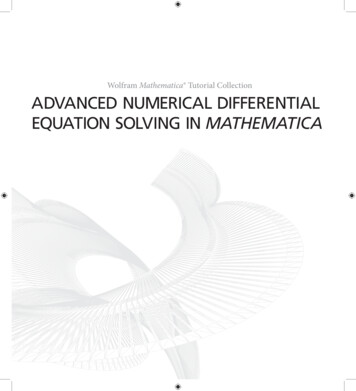
CHAPTER 1Approximation and Interpolation1. Introduction and PreliminariesThe problem we deal with in this chapter is the approximation of a given function bya simpler function. This has many possible uses. In the simplest case, we might want toevaluate the given function at a number of points, and an algorithm for this, we constructand evaluate the simpler function. More commonly the approximation problem is only thefirst step towards developing an algorithm to solve some other problem. For example, analgorithm to compute a definite integral of the given function might consist of first computingthe simpler approximate function, and then integrating that.To be more concrete we must specify what sorts of functions we seek to approximate(i.e., we must describe the space of possible inputs) and what sorts of simpler functions weallow. For both purposes, we shall use a vector space of functions. For example, we mightuse the vector space C(I), the space of all continuous functions on the closed unit intervalI [0, 1], as the source of functions to approximate, and the space Pn (I), consisting of allpolynomial functions on I of degree at most n, as the space of simpler functions in which toseek the approximation. Then, given f C(I), and a polynomial degree n, we wish to findp Pn (I) which is close to f .Of course, we need to describe in what sense the simpler functions is to approximate thegiven function. This is very dependent on the application we have in mind. For example, ifwe are concerned about the maximum error across the interval, the dashed line on the left ofFigure 1.1 shows the best cubic polynomial approximation to the function plotted with thesolid line. However if we are concerned about integrated quantities, the approximation onthe right of the figure may be more appropriate (it is the best approximation with respectto the L2 or root–mean–square norm).We shall always use a norm on the function space to measure the error. Recall that anorm on a vector space V is mapping which associated to any f V a real number, oftendenoted kf k which satisfies the homogeneity condition kcf k c kf k for c R and f V ,the triangle inequality kf gk kf k kgk, and which is strictly positive for all non-zerof . If we relax the last condition to just kf k 0, we get a seminorm.Now we consider some of the most important examples. We begin with the finite dimensional vector space Rn , mostly as motivation for the case of function spaces.(1) On Rn we may put the lp norm, 1 p kxklp n Xp xi 1/p,kxkl sup xi .1 i ni 11
21. APPROXIMATION AND INTERPOLATIONFigure 1.1. The best approximation depends on the norm in which we measure the error.(The triangle inequality for the lp norm is called Minkowski’s inequality.) If wi 0, i 1, . . . , n, we can define the weighted lp normsn X 1/pkxkw,p wi xi p, kxkw, sup wi xi .1 i ni 1The various lp norms are equivalent in the sense that there is a positive constant C such thatkxklp Ckxklq ,kxklq Ckxklp ,x Rn .Indeed all norms on a finite dimensional space are equivalent. Note also that if we extend theweighted lp norms to allow non-negative weighting functions which are not strictly positive,we get a seminorm rather than a norm.(2) Let I [0, 1] be the closed unit interval. We define C(I) to be the space of continuousfunctions on I with the L norm,kf kL (I) sup f (x) .x IObviously we can generalize I to any compact interval, or in fact any compact subset of Rn(or even more generally). Given a positive bounded weighting function w : I (0, ) wemay define the weighted normkf kw, sup[w(x) f (x) ].x IIf we allow w to be zero on parts of I this still defines a seminorm. If we allow w to beunbounded, we still get a norm (or perhaps a seminorm if w vanishes somewhere), but onlydefined on a subspace of C(I).(3) For 1 p we can define the Lp (I) norm on C(I), or, given a positive weightfunction, a weighted Lp (I) norm. Again the triangle inequality, which is not obvious, iscalled Minkowski’s inequality. For p q, we have kf kLp kf kLq , but these norms arenot equivalent. For p this space is not complete in that there may exist a sequenceof functions fn in C(I) and a function f not in C(I) such that kfn f kLp goes to zero.Completing C(I) in the Lp (I) norm leads to function space Lp (I). It is essentially the spaceof all functions for which kf kp , but there are some subtleties in defining it rigorously.
1. INTRODUCTION AND PRELIMINARIES3(4) On C n (I), n N the space on n times continuously differentiable functions, we have(n)n kfthe seminorm f W k . The norm in C n (I) is given byn sup f W k .kf kW 0 k n(5) If n N, 1 p , we define the Sobolev seminorm f Wpn : kf (n) kLp , and theSobolev norm bynXkf kWpn : ( f pW k )1/p .pk 0We are interested in the approximaton of a given function f , defined, say on the unitinterval, by a “simpler” function, namely by a function belonging to some particular subspaceS of C n which we choose. (In particular, we will be interested in the case S Pn (I), thevector space of polynomials of degree at most n restricted to I.) We shall be interested intwo sorts of questions: How good is the best approximation? How good are various computable approximation procedures?In order for either of these questions to make sense, we need to know what we mean bygood. We shall always use a norm (or at least a seminorm) to specify the goodness of theapproximation. We shall take up the first question, the theory of best approximation, first.Thus we want to know about inf p P f p for some specified norm.Various questions come immediately to mind: Does there exist p P minimizing kf pk?Could there exist more than one minimizer?Can the (or a) minimizer be computed?What can we say about the error?The answer to the first question is affirmative under quite weak hypotheses. To see this,we first prove a simple lemma.Lemma 1.1. Let there be given a normed vector space X Pand n 1 elements f0 , . . . , fnnof X. Then the function φ : R R given by φ(a) kf0 ni 1 ai fi k is continuous.Proof. We easily deduce from the triangle inequality that kf k kgk kf gk.ThereforeXXX φ(a) φ(b) (ai bi )fi ai bi kfi k M ai bi ,where M maxkfi k. Theorem 1.2. Let there be given a normed vector space X and a finite dimensionalvector subspace P . Then for any f X there exists p P minimizing kf pk.PProof. Let f1 , . . . , fn be a basis for P . The map a 7 k ni 1 ai fi k is then a norm onRn . Hence it is equivalent to any other norm, and so the setXS { a Rn ai f i 2kf k },
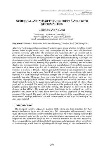
41. APPROXIMATION AND INTERPOLATIONPis closed and bounded. We wish to show that the function φ : Rn R, φ(a) kf ai fi kattains its minimum on Rn . By the lemma this is a continuous function, so it certainlyattains a minimum on S, say at a0 . But if a Rn \ S, thenXφ(a) kai fi k kf k kf k φ(0) φ(a0 ).This shows that a0 is a global minimizer. A norm is called strictly convex if its unit ball is strictly convex. That is, if kf k kgk 1,f 6 g, and 0 θ 1 implies that kθf (1 θ)gk 1. The Lp norm is strictly convex for1 p , but not for p 1 or .Theorem 1.3. Let X be a strictly convex normed vector space, P a subspace, f X,and suppose that p and q are both best approximations of f in P . Then p q.Proof. By hypothesis kf pk kf qk inf r P kf rk. By strict convexity, if p 6 q,thenkf (p q)/2k k(f p)/2 (f q)/2k inf kf rk,r Pwhich is impossible. RExercise: a) Using the integral (kf k2 g kgk2 f )2 , prove the Cauchy-Schwarz inequality:R1if f, g C(I) then 0 f (x)g(x) dx kf k2 kgk2 with equality if and only if f 0, g 0, orf cg for some constant c 0. b) Use this to show that the triangle inequality is satisfiedby the 2-norm, and c) that the 2-norm is strictly convex.2. Minimax Polynomial Approximation2.1. The Weierstrass Approximation Theorem and the Bernstein polynomials. We shall now focus on the case of best approximation by polynomials of degree at mostn measured in the L norm (minimax approximation). Below we shall look at the case ofbest approximation by polynomials measured in the L2 norm (least squares approximation).We first show that arbitrarily good approximation is possible if the degree is high enough.Theorem 1.4 (Weierstrass Approximation Theorem). Let f C(I) and 0. Thenthere exists a polynomial p such that kf pk .We shall give a constructive proof due to S. Bernstein. For f C(I), n 1, 2, . . ., defineBn f Pn (I) by nXkn kBn f (x) fx (1 x)n k .nkk 0Nown Xnk 0kxk (1 x)n k [x (1 x)]n 1,so for each x, Bn f (x) is a weighted average of the n 1 values f (0), f (1/n), . . . , f (1). Forexample,B2 f (x) f (0)(1 x)2 2f (1/2)x(x 1) f (1)x2 . The weighting functions nk xk (1 x)n k entering the definition of Bn f are shown in Figure 1.2. Note that for x near k/n, the weighted average weighs f (k/n) more heavily than
2. MINIMAX POLYNOMIAL APPROXIMATION5Figure 1.2. The Bernstein weighting functions for n 5 and n .40.60.81other values. Notice also that B1 f (x) f (0)(1 x) f (1)x is just the linear polynomialinterpolating f at x 0 and x 1.Now Bn is a linear map of C(I) into Pn . Moreover, it follows immediately from thepositivity of the Bernstein weights that Bn is a positive operator in the sense that Bn f 0on I if f 0 on I. Now we wish to show that Bn f converges to f in C(I) for all f C(I).Remarkably, just using the fact Bn is a positive linear operator, this follows from the muchmore elementary fact that Bn f converges to f in C(I) for all f P2 (I). This latter factwe can verify by direct computation. Let fi (x) xi , so we need to show that Bn fi fi ,i 0, 1, 2. (By linearity the result then extends to all f P2 (I). We know thatn Xn k n ka b (a b)n ,kk 0and by differentiating twice with respect to a we get also that nnXXk n k n kk(k 1) n k n kn 1a b a(a b) ,a b a2 (a b)n 2 .n kn(n 1) kk 0k 0Setting a x, b 1 x, expandingk(k 1)n k21 k n(n 1)n 1 n2 n 1 nin the last equation, and doing a little algebra we get thatn 11f2 f1 ,Bn f0 f0 , Bn f1 f1 , Bn f2 nnfor n 1, 2, . . .Now we derive from this convergence for all continuous functions.Theorem 1.5. Let B1 , B2 , . . . be any sequence of linear positive operators from C(I) intoitself such that Bn f converges uniformly to f for f P2 . Then Bn f converges uniformly tof for all f C(I).Proof. The idea is that for any f C(I) and x0 I we can find a quadratic functionq that is everywhere greater than f , but for which q(x0 ) is close to f (x0 ). Then, for nsufficiently large Bn q(x0 ) will be close to q(x0 ) and so close to f (x0 ). But Bn f must be lessthan Bn q. Together these imply that Bn f (x0 ) can be at most a little bit larger than f (x0 ).Similarly we can show it can be at most a little bit smaller than f (x0 ).
61. APPROXIMATION AND INTERPOLATIONSince f is continuous on a compact set it is uniformly continuous. Given 0, chooseδ 0 such that f (x1 ) f (x2 ) if x1 x2 δ. For any x0 , setq(x) f (x0 ) 2kf k (x x0 )2 /δ 2 .Then, by checking the cases x x0 δ and x x0 δ separately, we see that q(x) f (x)for all x I.Writing q(x) a bx cx2 we see that we can write a , b , c M with M dependingon kf k, , and δ, but not on x0 . Now we can choose N sufficiently large that kfi Bn fi k , i 0, 1, 2,Mfor n N , where fi xi . Using the triangle inequality and the bounds on the coefficientsof q, we get kq Bn qk 3 . ThereforeBn f (x0 ) Bn q(x0 ) q(x0 ) 3 f (x0 ) 4 .Thus we have shown: given f C(I) and 0 there exists N 0 such that Bn f (x0 ) f (x0 ) 4 for all n N and all x0 I.The same reasoning, but using q(x) f (x0 ) 2kf k (x x0 )2 /δ 2 implies thatBn f (x0 ) f (x0 ) 4 , and together these complete the theorem. From a practical point of view the Bernstein polynomials yield an approximation procedure which is very robust but very slow. By robust we refer to the fact that the procedureconvergence for any continuous function, no matter how bad (even, say, nowhere differentiable). Moreover if the function is C 1 then not only does Bn f converge uniformly tof , but (Bn f )0 converges uniformly to f 0 (i.e., we have convergence of Bn f in C 1 (I), andsimilarly if f admits more continuous derivatives. However, even for very nice functionsthe convergence is rather slow. Even for as simple a function as f (x) x2 , we saw thatkf Bn f k O(1/n). In fact, refining the argument of the proof, one can show that thissame linear rate of convergence holds for all C 2 functions f :1 00kf Bn f k kf k, f C 2 (I).8nthis bound holds with equality for f (x) x2 , and so cannot be improved. This slow rateof convergence makes the Bernstein polynomials impractical for most applications. SeeFigure 1.3 where the linear rate of convergence is quite evident.2.2. Jackson’s theorems for trigonometric polynomials. In the next sections weaddress the question of how quickly a given continuous function can be approximated by asequence of polynomials of increasing degree. The results were mostly obtained by DunhamJackson in the first third of the twentieth century and are known collectively as Jackson’stheorems. Essentially they say that if a function is in C k then it can be approximated by asequence of polynomials of degree n in such a way that the error is at most C/nk as n .Thus the smoother a function is, the better the rate of convergence.Jackson proved this sort of result both for approximation by polynomials and for approximation by trigonometric polynomials (finite Fourier series). The two sets of resultsare intimately related, as we shall see, but it is easier to get started with the results fortrigonometric polynomials, as we do now.
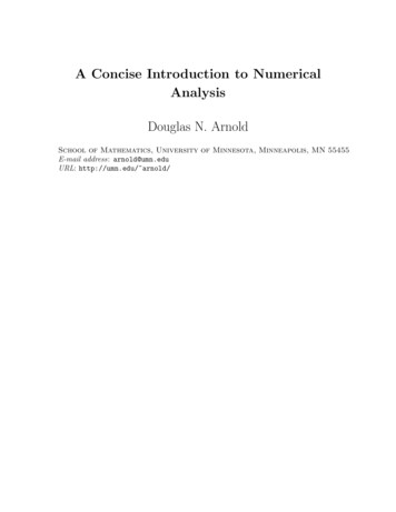
2. MINIMAX POLYNOMIAL APPROXIMATION7Figure 1.3. Approximation to the function sin x on the interval [0, 8] byBernstein polynomials of degrees 1, 2, 4, . . . , 32.1320.8160.60.4180.240 0.22 0.4 0.6 0.8 1012345678kthe set ofLet C2π be the set of 2π-periodic continuous functions on the real line, and C2π2π-periodic functions which belong to C k (R). We shall investigate the rate of approximationof such functions by trigonometric polynomials of degree n. By these we mean linear combinations of the n 1 functions 1, cos kx, sin kx, k 1, . . . , n, and we denote by Tn the spaceof all trigonometric polynomials of degree n, i.e., the span of these of the 2n 1 functions.Using the relations sin x (eix e ix )/(2i), cos x (eix e ix )/2, we can equivalently writeTn {nXck eikx ck C, c k c̄k }.k n1Our immediate goal is the Jackson Theorem for the approximation of functions in C2πby trigonometric polynomials.1Theorem 1.6. If f C2π, theninf kf pk p Tnπkf 0 k.2(n 1)(We are suppressing the subscript on the L norm, since that is the only norm thatwe’ll be using in this section.) The proof will be quite explicit. We startR π by 0writing f (x) as0an integral of f times an appropriate kernel. Consider the integral π yf (x π y) dy.Integrating by parts and using the fact that f is 2π-periodic we getZ πZ π0yf (x π y) dy f (x π y) dx 2πf (x). π πThe integral on the right-hand side is just the integral of f over one period (and so independent of x), and we can rearrange to getZ π1 f (x) f yf 0 (x π y) dy,2π π
81. APPROXIMATION AND INTERPOLATIONFigure 1.4. The interpolant qn Tn of the sawtooth function for n 2 andn 10.3300 3 3 pi0pi pi0piwhere f is the average value of f over any period. Now supposeP we replace the function yin the last integral with a trigonometric polynomial qn (y) nk n ck eiky . This givesZ πZ πZ πnX00ckeik(y π) f 0 (y) dy e ikx ,qn (y)f (x π y) dy qn (y π x)f (y) dy π πk n πwhich is a trigonometric polynomial of degree at most n in x. ThusZ π1pn (x) : f qn (y)f 0 (x π y) dy Tn ,2π πand pn (x) is close to f (x) if q(y) is close to y on [ π, π]. SpecificallyZ πZ π110(1.1) f (x) pn (x) [y qn (y)]f (x π y) dy y qn (y) dykf 0 k.2π π2π πThus to obtain a bound on the error, we need only give a bound on the L1 error in trigonometric polynomial approximation to the function g(y) y on [ π, π]. (Note that, since weare working in the realm of 2π periodic functions, g is the sawtooth function.)Lemma 1.7. There exists qn Tn such thatZ π x qn (x) dx ππ2.n 1This we shall prove quite explicitly, by exhibiting qn . Note that the Jackson theorem,Theorem 1.6 follows directly from (1.1) and the lemma.Proof. To prove the Lemma, we shall determine qn Tn by the 2n 1 equations πkπkqn , k n, . . . , n.n 1n 1That, is, qn interpolates the saw tooth function at the n 1 points with abscissas equal toπk/(n 1). See Figure 1.4.This defines qn uniquely. To see this it is enough to note that if a trigonometric polynomialof degree n vanishes at 2n 1 distinct points in [ π, π) it vanishes identically. This is
2. MINIMAX POLYNOMIAL APPROXIMATION9PPso because if nk n ck eikx vanishes at xj , j n, . . . , n, then z n nk n ck z k , which is apolynomial of degree 2n, vanishes at the 2n 1 distinct complex numbers eixj , so is identicallyzero, which implies that all the ck vanish.Now qn is odd, since replacing qn (x) withP qn ( x) would give another solution, whichthen must coincide with qn . Thus qn (x) nk 1 bk sin kx.To get a handle on the error x qn (x) we first note that by construction this functionhas 2n 1 zeros in ( π, π), namely at the points πk/(n 1). It can’t have any other zeros orany double zeros in this interval, for if it did Rolle’s Theorem would imply that its derivative1 qn0 Tn , would have 2n 1 zeros in the interval, and, by the argument above, wouldvanish identically, which is not possible (it has mean value 1). Thus qn changes sign exactlyat the points πk/(n 1).Define the piecewise constant functions(x) ( 1)k ,ThenZkπ(k 1)π x ,n 1n 1πk Z.Z x qn (x) dx [x qn (x)]s(x) dx. πBut, as we shall show in a moment,Z(1.2)sin kx s(x) dx 0,and it is easy to calculateRk 1, . . . , n,xs(x) dx π 2 /(n 1). ThusZ ππ2 x qn (x) dx ,n 1 πas claimed.We complete the proof of the lemma by verifying (1.2). Let I denote the integral inquestion. ThenZZππI s(x ) sin kx dx s(x) sin k(x ) dxn 1n 1Z kπ kπ cos() s(x) sin kx dx cos()I.n 1n 1) 1, this implies that I 0.Since cos( kπn 1 1Having proved a Jackson Theorem in C2π, we can use a bootstrap argument to show thatif f is smoother, then the rate of convergence of the best approximation is better. This iskthe Jackson Theorem in C2π.k, some k 0, thenTheorem 1.8. If f C2π k πinf kf pk kf (k) k.p Tn2(n 1)
101. APPROXIMATION AND INTERPOLATIONProof. We shall use induction on k, the case k 1 having been established. Assumingthe result, we must show it holds when k is replaced by k 1. Now let q Tn be arbitrary.Then kπinf kf pk inf kf q pk k(f q)(k) k,p Tnp Tn2(n 1)by the inductive hypothesis. Since q is arbitrary and { p(k) p Tn } T̂n , k k πππ(k)inf kf pk kf (k 1) k.inf kf rk p Tn2(n 1) r T̂n2(n 1) 2(n 1) 2.3. Jackson theorems for algebraic polynomials. To obtain the Jackson theoremsfor algebraic polynomials we use the following transformation. Given f : [ 1, 1] R defineg : R R by g(θ) f (cos θ). Then g is 2π-periodic and even. This transformation is a linear1isometry (kgk kf k). Note that if f C 1 ([ 1, 1]) then g C2πand g 0 (θ) f 0 (cos θ) sin θ,00nix ixso kg k kf k. Also if f (x) x , then g(θ) [(e e )/2]n which is a trigonometricpolynomial of degree at most n. Thus this transformation maps Pn ([ 1, 1]) to the Tneven ,the subspace of even functions in Tn , or, equivalently, the span of cos kx, k 0, . . . , n. Sincedim Tneven dim Pn ([ 1, 1]) n 1, the transformation is in fact an isomorphism.1:The Jackson theorem in C 1 ([ 1, 1]) follows immediately from that in C2πTheorem 1.9. If f C 1 ([ 1, 1]), theninf kf pk p Pnπkf 0 k.2(n 1)1Proof. Define g(θ) f (cos θ) so g C2π. Since g is even, inf q Tneven kg qk inf q Tn kg qk. (If the second infimum is achieved by q(θ), then it is also achieved by q( θ), then usethe triangle inequality to show it is also achieved by the even function [q(θ) q( θ)]/2.)Thusππinf kf pk inf kg qk kg 0 k kf 0 k.p Pnq Tn2(n 1)2(n 1) kYou can’t derive the Jackson theorem in C k ([ 1, 1]) from that in C2π(since we can’t(k)(k)bound kg k by kf k for k 2), but we can use a bootstrap argument directly. We knowthatπinf kf pk inf inf kf q pk infkf 0 q 0 k.p Pnq Pn p Pnq Pn 2(n 1)Assuming n 1, q 0 is an arbitrary element of Pn 1 and so we haveπππ 00inf kf pk infkf 0 pk kf k.p Pnp Pn 1 2(n 1)2(n 1) 2nBut now we can apply the same argument to getπππinf kf pk kf 000 k,p Pn2(n 1) 2n 2(n 1)as long as n 2. Continuing in this way we getckinf kf pk kf (k) kp Pn(n 1)n(n 1) . . . (n k 2)
2. MINIMAX POLYNOMIAL APPROXIMATION11if f C k and n k 1, with ck (π/2)k . To state the result a little more compactly weanalyze the product M (n 1)n(n 1) . . . (n k 2). Now if n 2(k 2) then eachfactor is at least n/2, so M nk /2k . Alsodk : nk ,k 1 n 2(k 2) (n 1)n(n 1) . . . (n k 2)maxso, in all, nk ek M where ek max(2k , dk ). Thus we have arrived at the Jackson theoremin C k :Theorem 1.10. Let k be a positive integer, n k 1 an integer. Then there exists aconstant c depending only on k such thatinf kf pk p Pnc (k)kf k.nkfor all f C k ([ 1, 1]).2.4. Polynomial approximation of analytic functions. If a function is C theJackson theorems show that the best polynomial approximation converges faster than anypower of n. If we go one step farther and assume that the function is analytic (i.e., itspower series converges at every point of the interval including the end points), we can proveexponential convergence.We will first do the periodic case and show that the Fourier series for an analytic periodicfunction converges exponentially, and then use the Chebyshev transform to carry the resultover to the algebraic case.A real function on an open interval is called real analytic if the function is C and forevery point in the interval the Taylor series for the function about that point converges tothe function in some neighborhood of the point. A real function on a closed interval J isreal analytic if it is real analytic on some open interval containing J.It is easy to see that a real function is real analytic on an interval if and only if it extendsto an analytic function on a neighborhood of the interval in the complex plane.Suppose that g(z) is real analytic and 2π-periodic on R. Since g is smooth and periodicits Fourier series,Z π X1inxg(x) an e , an g(x)e inx dx,2π πn converges absolutely and uniformly on R. Since g is real analytic, it extends to an analyticfunction on the strip Sδ : { x iy x, y R, y δ } for some δ 0. Using analyticitywe see that we can shift the segment [ π, π] on which we integrate to define the Fouriercoefficients upward or downward a distance δ in the complex plane:Z πZ1e nδ π in(x iδ)an g(x iδ)edx g(x iδ)e inx dx.2π π2π πThus an kgkL (Sδ ) e δ n and we have shown that the Fourier coefficients of a real analyticperiodic function decay exponentially.
121. APPROXIMATION AND INTERPOLATIONNow consider the truncated Fourier series q(z) Pikz, so for any real z k n ak e g(z) q(z) X ak 2kgk k nL (S Xδ)k n 1Pnk ne δkak eikz Tn . Then g(z) q(z) 2e δ kgkL (Sδ ) e δn . δ1 eThus we have proven:Theorem 1.11. Let g be 2π-periodic and real analytic. Then there exist positive constantsC and δ so thatinf kg qk Ce δn .q TnThe algebraic case follows immediately from the periodic one. If f is real analytic on[ 1, 1], then g(θ) f (cos θ) is 2π-periodic and real analytic. Since inf q Tn kg qk inf q Tneven kg qk inf p Pn kf pk , we can apply the previous result to bound the latterquantity by Ce δn .Theorem 1.12. Let f be real analytic on a closed interval. Then there exist positiveconstants C and δ so thatinf kf pk Ce δn .p Pn2.5. Characterization of the minimax approximant. Having established the rateof approximation afforded by the best polynomial approximation with respect to the L norm, in this section we derive two conditions that characterize the best approximation.We will use these results to show that the best approximation is unique (recall that ouruniqueness theorem in the first section only applied to strictly convex norms, and so excludedthe case of L approximation). The results of this section can also be used to design iterativealgorithms which converge to the best approximation, but we shall not pursue that, becausethere are approximations which yield nearly as good approximation in practice as the bestapproximation but which are much easier to compute.The first result applies very generally. Let J be an compact subset of Rn (or even ofa general Hausdorff topological space), and let P be any finite dimensional subspace ofC(J). For definiteness you can think of J as a closed interval and P as the space Pn (J) ofpolynomials of degree at most n, but the result doesn’t require this.Theorem 1.13 (Kolmogorov Characterization Theorem). Let f C(J), P a finitedimensional subspace of C(J), p P . Then p is a best approximation to f in P if and onlyif no element of P has the same sign as f p on its extreme set.Proof. First we note that p is a best approximation to f in P if and only if 0 is a bestapproximation to g : f p in P . So we need to show that 0 is a best approximation to gif and only if no element q of P has the same sign as g on its extreme set.First suppose that 0 is not a best approximation. Then there exists q P such thatkg qk kgk. Now let x be a point in the extreme set of g. Unless sign q(x) sign g(x), g(x) q(x) g(x) kgk, which is impossible. Thus q has the same sign of as g on itsextreme set.The converse direction is trickier, but the idea is simple. If q has the same sign of asg on its extreme set and we subtract a sufficiently small positive multiple of q from g, the
2. MINIMAX POLYNOMIAL APPROXIMATION13difference will be of strictly smaller magnitude than g near the extreme set. And if themultiple that we subtract is small enough the difference will also stay below the extremevalue away from the extreme set. Thus g q will be smaller than g for small enough, sothat 0 is not the best approximation.Since we may replace q by q/kqk we can assume from the outset that kqk 1. Let δ 0be the minimum of qg on the extreme set, and set S { x J q(x)g(x) δ/2}, so that Sis an open set containing the extreme set. Let M maxJ\S g kgk.Now on S, qg δ/2, so g q 2 g 2 2 qg 2 q 2 kgk2 δ 2 kgk2 (δ ),and so if 0 δ then kg qk ,S kgk.On J \ S, g q M , so if 0 kgk M , kg qk ,J\S kgk. Thus for anypositive sufficiently small kg qk kgk on J. While the above result applies to approximation by any finite dimensional subspace P
2. The ve-point discretization of the Laplacian 153 3. Finite element methods 162 4. Di erence methods for the heat equation 177 5. Di erence methods for hyperbolic equations 183 6. Hyperbolic conservation laws 189 Exercises 190 Chapter 7. Some Iterative Methods of Numerical Linear Algebra 193 1. Introduction 193 2. Classical iterations 194 3 .