Transcription
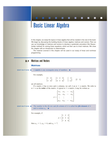
Basic Linear AlgebraIn this chapter, we study the topics in linear algebra that will be needed in the rest of the book.We begin by discussing the building blocks of linear algebra: matrices and vectors. Then weuse our knowledge of matrices and vectors to develop a systematic procedure (the Gauss–Jordan method) for solving linear equations, which we then use to invert matrices. We closethe chapter with an introduction to determinants.The material covered in this chapter will be used in our study of linear and nonlinearprogramming.2.1Matrices and VectorsMatricesDEFINITION A matrix is any rectangular array of numbers. For example, 3 4 ,12 4125 2 ,3,61[21]are all matrices.If a matrix A has m rows and n columns, we call A an m n matrix. We refer tom n as the order of the matrix. A typical m n matrix A may be written as a11a21A am1DEFINITION a1n a2n a mna12a22 am2The number in the ith row and jth column of A is called the ijth element of Aand is written aij. For example, if 1A 47then a11 1, a23 6, and a31 7.258369
Sometimes we will use the notation A [aij] to indicate that A is the matrix whoseijth element is aij.DEFINITION Two matrices A [aij] and B [bij] are equal if and only if A and B are of thesame order and for all i and j, aij bij. For example, ifA 3 4 12B and w z x ythen A B if and only if x 1, y 2, w 3, and z 4.VectorsAny matrix with only one column (that is, any m 1 matrix) may be thought of as a columnvector. The number of rows in a column vector is the dimension of the column vector. Thus, 2 1may be thought of as a 2 1 matrix or a two-dimensional column vector. Rm will denotethe set of all m-dimensional column vectors.In analogous fashion, we can think of any vector with only one row (a 1 n matrix asa row vector. The dimension of a row vector is the number of columns in the vector. Thus,[9 2 3] may be viewed as a 1 3 matrix or a three-dimensional row vector. In this book,vectors appear in boldface type: for instance, vector v. An m-dimensional vector (either rowor column) in which all elements equal zero is called a zero vector (written 0). Thus,[00]and 0 0are two-dimensional zero vectors.Any m-dimensional vector corresponds to a directed line segment in the m-dimensionalplane. For example, in the two-dimensional plane, the vectoru 2 1corresponds to the line segment joining the point 0 0to the point 2 1The directed line segments corresponding tou are drawn in Figure 1.12CHAPTER2 Basic Linear Algebra 2 ,1v 3 ,1w 1 2
x2u 12v 1–3w –1–232(1, 2)u1–2–11wx12–1v(–1, –2)FIGURE–21Vectors Are DirectedLine Segments–3(1, –3)The Scalar Product of Two VectorsAn important result of multiplying two vectors is the scalar product. To define the scalar product of two vectors, suppose we have a row vector u [u1 u2 un] and a column vector v1v2v vnof the same dimension. The scalar product of u and v (written u v) is the numberu1v1 u2v2 unvn.For the scalar product of two vectors to be defined, the first vector must be a row vector and the second vector must be a column vector. For example, ifu [123]and 2v 12then u v 1(2) 2(1) 3(2) 10. By these rules for computing a scalar product, ifu 2 1andv [2 3]then u v is not defined. Also, ifu [123]andv 4 3then u v is not defined because the vectors are of two different dimensions.Note that two vectors are perpendicular if and only if their scalar product equals 0.Thus, the vectors [1 1] and [1 1] are perpendicular.We note that u v u v cos u, where u is the length of the vector u and u is theangle between the vectors u and v.2 . 1 Matrices and Vectors13
Matrix OperationsWe now describe the arithmetic operations on matrices that are used later in this book.The Scalar Multiple of a MatrixGiven any matrix A and any number c (a number is sometimes referred to as a scalar),the matrix cA is obtained from the matrix A by multiplying each element of A by c. Forexample,A if 1 0 ,12then3A 3 0 36For c 1, scalar multiplication of the matrix A is sometimes written as A.Addition of Two MatricesLet A [aij] and B [bij] be two matrices with the same order (say, m n). Then thematrix C A B is defined to be the m n matrix whose ijth element is aij bij. Thus,to obtain the sum of two matrices A and B, we add the corresponding elements of A andB. For example, ifA 012 1 31B and 1 2 321 1 thenA B 1 1 0 22 2 3 30 1 1 1 12 00 0.0This rule for matrix addition may be used to add vectors of the same dimension. For example, if u [1 2] and v [2 1], then u v [1 2 2 1] [3 3]. Vectorsmay be added geometrically by the parallelogram law (see Figure 2).We can use scalar multiplication and the addition of matrices to define the conceptof a line segment. A glance at Figure 1 should convince you that any point u in them-dimensional plane corresponds to the m-dimensional vector u formed by joining theorigin to the point u. For any two points u and v in the m-dimensional plane, the linesegment joining u and v (called the line segment uv) is the set of all points in them-dimensional plane that correspond to the vectors cu (1 c)v, where 0 c 1(Figure 3). For example, if u (1, 2) and v (2, 1), then the line segment uv consistsx2v u u v 2 11 23 33(3, 3)2(1, 2)u vu1(2, 1)v(0, 0)FIGURE21Addition of Vectors14CHAPTER2 Basic Linear Algebra23x1
x2u c 1212c c 0v1FIGURE3Line Segment Joiningu (1, 2) andv (2, 1)1x12of the points corresponding to the vectors c[1 2] (1 c)[2 1] [2 c 1 c],where 0 c 1. For c 0 and c 1, we obtain the endpoints of the line segment uv;for c 12 , we obtain the midpoint (0.5u 0.5v) of the line segment uv.Using the parallelogram law, the line segment uv may also be viewed as the points corresponding to the vectors u c(v u), where 0 c 1 (Figure 4). Observe that forc 0, we obtain the vector u (corresponding to point u), and for c 1, we obtain thevector v (corresponding to point v).The Transpose of a MatrixGiven any m n matrix a11a21A am1a12a22 am2 a1n a2n amnthe transpose of A (written AT) is the n m matrix a11a12TA a1na21a22 a2n am1 am2 a mnx2u c 0c u12c 1vvx1–uFIGUREv – u4Representation of LineSegment uv2 . 1 Matrices and Vectors15
Thus, AT is obtained from A by letting row 1 of A be column 1 of AT, letting row 2 of Abe column 2 of AT, and so on. For example, 1A 4if 253,6Observe that (AT)T A. Let B [1BT 2 1 1A 23Tthen4562]; thenand(BT)T [12] BAs indicated by these two examples, for any matrix A, (AT)T A.Matrix MultiplicationGiven two matrices A and B, the matrix product of A and B (written AB) is defined if andonly ifNumber of columns in A number of rows in B(1)For the moment, assume that for some positive integer r, A has r columns and B has rrows. Then for some m and n, A is an m r matrix and B is an r n matrix.DEFINITION The matrix product C AB of A and B is the m n matrix C whose ijthelement is determined as follows:ijth element of C scalar product of row i of A column j of B (2)If Equation (1) is satisfied, then each row of A and each column of B will have thesame number of elements. Also, if (1) is satisfied, then the scalar product in Equation (2)will be defined. The product matrix C AB will have the same number of rows as A andthe same number of columns as B.EXAMPLE1Matrix MultiplicationCompute C AB for 1A 2Solution 23and 1B 21132Because A is a 2 3 matrix and B is a 3 2 matrix, AB is defined, and C will be a2 2 matrix. From Equation (2),CHAPTER 112] 2 1(1) 1(2) 2(1) 51c12 [1112] 3 1(1) 1(3) 2(2) 82c21 [2113] 2 2(1) 1(2) 3(1) 71c11 [116112 Basic Linear Algebra
1c22 [2 1 3] 3 2(1) 1(3) 3(2) 11258C AB 7 11 EXAMPLE2 Column Vector Times Row VectorFind AB forA Solution 4 3B [1and2]Because A has one column and B has one row, C AB will exist. From Equation (2), weknow that C is a 2 2 matrix withc11 3(1) 3c12 3(2) 6c21 4(1) 4c22 4(2) 8Thus,C EXAMPLE3 4 8 36Row Vector Times Column VectorCompute D BA for the A and B of Example 2.SolutionIn this case, D will be a 1 1 matrix (or a scalar). From Equation (2),d11 [1 4 1(3) 2(4) 112]3Thus, D [11]. In this example, matrix multiplication is equivalent to scalar multiplication of a row and column vector.Recall that if you multiply two real numbers a and b, then ab ba. This is called thecommutative property of multiplication. Examples 2 and 3 show that for matrix multiplication, it may be that AB BA. Matrix multiplication is not necessarily commutative. (Insome cases, however, AB BA will hold.)EXAMPLE4Undefined Matrix ProductShow that AB is undefined if 1A 3Solution24and 1B 01112This follows because A has two columns and B has three rows. Thus, Equation (1) is notsatisfied.2 . 1 Matrices and Vectors17
TA B L E1Gallons of Crude Oil Required to Produce 1 Gallonof gularLeaded3 41 42 31 31 43 4Many computations that commonly occur in operations research (and other branchesof mathematics) can be concisely expressed by using matrix multiplication.To illustratethis, suppose an oil company manufactures three types of gasoline: premium unleaded,regular unleaded, and regular leaded. These gasolines are produced by mixing two typesof crude oil: crude oil 1 and crude oil 2. The number of gallons of crude oil required tomanufacture 1 gallon of gasoline is given in Table 1.From this information, we can find the amount of each type of crude oil needed tomanufacture a given amount of gasoline. For example, if the company wants to produce10 gallons of premium unleaded, 6 gallons of regular unleaded, and 5 gallons of regularleaded, then the company’s crude oil requirements would beCrude 1 required ( 34 ) (10) ( 23 ) (6) ( 14 ) 5 12.75 gallonsCrude 2 required ( 14 ) (10) ( 13 ) (6) ( 34 ) 5 8.25 gallonsMore generally, we definepU gallons of premium unleaded producedrU gallons of regular unleaded producedrL gallons of regular leaded producedc1 gallons of crude 1 requiredc2 gallons of crude 2 requiredThen the relationship between these variables may be expressed byc1 ( 34 ) pU ( 23 ) rU ( 14 ) rLc2 ( 14 ) pU ( 13 ) rU ( 34 ) rLUsing matrix multiplication, these relationships may be expressed by c1 c2 3 41 42 31 31 43 4 pUrUrLProperties of Matrix MultiplicationTo close this section, we discuss some important properties of matrix multiplication. Inwhat follows, we assume that all matrix products are defined.1Row i of AB (row i of A)B. To illustrate this property, let 1A 211 23andThen row 2 of the 2 2 matrix AB is equal to18CHAPTER2 Basic Linear Algebra 1B 21132
[2 13] 21113 [7211]This answer agrees with Example 1.2 Column j of AB A(column j of B). Thus, for A and B as given, the first columnof AB is11 1 252 2 1 371 Properties 1 and 2 are helpful when you need to compute only part of the matrix AB.3Matrix multiplication is associative. That is, A(BC) (AB)C. To illustrate, letA [1B 2], 4 5 ,23C 1 2Then AB [10 13] and (AB)C 10(2) 13(1) [33].On the other hand, 13 7BC so A(BC) 1(7) 2(13) [33]. In this case, A(BC) (AB)C does hold.Matrix multiplication is distributive. That is, A(B C) AB AC and (B C)D BD CD.4Matrix Multiplication with ExcelUsing the Excel MMULT function, it is easy to multiply matrices. To illustrate, let’s useExcel to find the matrix product AB that we found in Example 1 (see Figure 5 and fileMmult.xls). We proceed as follows:Mmult.xlsStep 1Enter A and B in D2:F3 and D5:E7, respectively.Step 2Select the range (D9:E10) in which the product AB will be computed.Step 3In the upper left-hand corner (D9) of the selected range, type the formula MMULT(D2:F3,D5:E7)Then hit Control Shift Enter (not just Enter), and the desired matrix product will becomputed. Note that MMULT is an array function and not an ordinary spreadsheet function. This explains why we must preselect the range for AB and use Control Shift Enter.FIGURE5AB1 7811232 . 1 Matrices and Vectors19
PROBLEMSGroup AGroup B 11 For A 47a Ad ATg BA258 36and9b 3Ae BT12B 0 1 , find:12c A 2Bf AB2 Only three brands of beer (beer 1, beer 2, and beer 3)are available for sale in Metropolis. From time to time,people try one or another of these brands. Suppose that atthe beginning of each month, people change the beer theyare drinking according to the following rules:30% of the people who prefer beer 1 switch to beer 2.20% of the people who prefer beer 1 switch to beer 3.30% of the people who prefer beer 2 switch to beer 3.30% of the people who prefer beer 3 switch to beer 2.10% of the people who prefer beer 3 switch to beer 1.For i 1, 2, 3, let xi be the number who prefer beer i atthe beginning of this month and yi be the number who prefer beer i at the beginning of next month. Use matrix multiplication to relate the following:3Prove that matrix multiplication is associative.4Show that for any two matrices A and B, (AB)T BT AT.5An n n matrix A is symmetric if A AT.a Show that for any n n matrix, AAT is a symmetric matrix.b Show that for any n n matrix A, (A AT) is asymmetric matrix.6 Suppose that A and B are both n n matrices. Showthat computing the matrix product AB requires n3multiplications and n3 n2 additions.7 The trace of a matrix is the sum of its diagonalelements.a For any two matrices A and B, show that trace(A B) trace A trace B.b For any two matrices A and B for which the productsAB and BA are defined, show that trace AB trace BA. y1y2y32.2x1x2x3Matrices and Systems of Linear EquationsConsider a system of linear equations given bya11x1 a12x2 a1nxn b1a21x1 a22x2 a2nxn b2 am1x1 am2x2 amnxn bm(3)In Equation (3), x1, x2, . . . , xn are referred to as variables, or unknowns, and the aij’sand bi’s are constants. A set of equations such as (3) is called a linear system of m equations in n variables.DEFINITION A solution to a linear system of m equations in n unknowns is a set of values forthe unknowns that satisfies each of the system’s m equations. To understand linear programming, we need to know a great deal about the propertiesof solutions to linear equation systems. With this in mind, we will devote much effort tostudying such systems.We denote a possible solution to Equation (3) by an n-dimensional column vector x,in which the ith element of x is the value of xi. The following example illustrates the concept of a solution to a linear system.20CHAPTER2 Basic Linear Algebra
EXAMPLE5Solution to Linear SystemShow thatx 2 1is a solution to the linear systemx1 2x2 52x1 x2 0(4)and thatx 1 x 2 3is not a solution to linear system (4).SolutionTo show that1is a solution to Equation (4), we substitute x1 1 and x2 2 in both equations and checkthat they are satisfied: 1 2(2) 5 and 2(1) 2 0.The vectorx 1 3is not a solution to (4), because x1 3 and x2 1 fail to satisfy 2x1 x2 0.Using matrices can greatly simplify the statement and solution of a system of linearequations. To show how matrices can be used to compactly represent Equation (3), let a12a11a21A am1a22 am2 a1n a2n , amnx1x2x , xnb1b2b bmThen (3) may be written asAx b(5)Observe that both sides of Equation (5) will be m 1 matrices (or m 1 column vectors). For the matrix Ax to equal the matrix b (or for the vector Ax to equal the vector b),their corresponding elements must be equal. The first element of Ax is the scalar productof row 1 of A with x. This may be written as x1[a11a12x2 a1n] a11x1 a12x2 a1nxn xnThis must equal the first element of b (which is b1). Thus, (5) implies that a11x1 a12x2 a1nxn b1. This is the first equation of (3). Similarly, (5) implies that the scalar2 . 2 Matrices and Systems of Linear Equations21
product of row i of A with x must equal bi, and this is just the ith equation of (3). Our discussion shows that (3) and (5) are two different ways of writing the same linear system. Wecall (5) the matrix representation of (3). For example, the matrix representation of (4) is 2 x 0 12 1x152Sometimes we abbreviate (5) by writingA b(6)If A is an m n matrix, it is assumed that the variables in (6) are x1, x2, . . . , xn. Then(6) is still another representation of (3). For instance, the matrix 101211321 231represents the system of equationsx1 2x2 3x3 2x2 2x3 3x1 x2 x3 1PROBLEMGroup A1 Use matrices to represent the following system ofequations in two different ways:2.3x1 x2 42x1 x2 6x1 3x2 8The Gauss–Jordan Method for Solving Systems of Linear EquationsWe develop in this section an efficient method (the Gauss–Jordan method) for solving asystem of linear equations. Using the Gauss–Jordan method, we show that any system oflinear equations must satisfy one of the following three cases:Case 1The system has no solution.Case 2The system has a unique solution.Case 3The system has an infinite number of solutions.The Gauss–Jordan method is also important because many of the manipulations used inthis method are used when solving linear programming problems by the simplex algorithm (see Chapter 4).Elementary Row OperationsBefore studying the Gauss–Jordan method, we need to define the concept of an elementary row operation (ERO). An ERO transforms a given matrix A into a new matrix Avia one of the following operations.22CHAPTER2 Basic Linear Algebra
Type 1 EROA is obtained by multiplying any row of A by a nonzero scalar. For example, if 1A 10231352 463then a Type 1 ERO that multiplies row 2 of A by 3 would yield 1A 302913152 4183Type 2 EROBegin by multiplying any row of A (say, row i) by a nonzero scalar c. For some j i, letrow j of A c(row i of A) row j of A, and let the other rows of A be the same as therows of A.For example, we might multiply row 2 of A by 4 and replace row 3 of A by 4(row 2of A) row 3 of A. Then row 3 of A becomes4 [1 356] [0123] [4132227]and 1A 1423133522 4627Type 3 EROInterchange any two rows of A. For instance, if we interchange rows 1 and 3 of A, weobtain 0A 11132253 364Type 1 and Type 2 EROs formalize the operations used to solve a linear equation system. To solve the system of equationsx1 x2 22x1 4x2 7(7)we might proceed as follows. First replace the second equation in (7) by 2(first equation in (7)) second equation in (7). This yields the following linear system:x1 x2 22x2 3(7.1)Then multiply the second equation in (7.1) by 12 , yielding the systemx1 x2 2x2 32 (7.2)Finally, replace the first equation in (7.2) by 1[second equation in (7.2)] first equation in (7.2). This yields the system2 . 3 The Gauss–Jordan Method for Solving Systems of Linear Equations23
1 2x2 32 x1 12 andx1 (7.3)System (7.3) has the unique solutionx2 32 . The systems (7), (7.1), (7.2),and (7.3) are equivalent in that they have the same set of solutions. This means that x1 13 and x2 is also the unique solution to the original system, (7).22If we view (7) in the augmented matrix form (A b), we see that the steps used to solve(7) may be seen as Type 1 and Type 2 EROs applied to A b. Begin with the augmentedmatrix version of (7): 2 4 7 112(7 )Now perform a Type 2 ERO by replacing row 2 of (7 ) by 2(row 1 of (7 )) row 2 of(7 ). The result is 0 2 3 112(7.1 )which corresponds to (7.1). Next, we multiply row 2 of (7.1 ) bysulting in1 2(a Type 1 ERO), re- 10112(7.2 )3 2which corresponds to (7.2). Finally, perform a Type 2 ERO by replacing row 1 of (7.2 )by 1(row 2 of (7.2 )) row 1 of (7.2 ). The result is 10011 23 2(7.3 )which corresponds to (7.3). Translating (7.3 ) back into a linear system, we obtain the system x1 12 and x2 32 , which is identical to (7.3).Finding a Solution by the Gauss–Jordan MethodThe discussion in the previous section indicates that if the matrix A b is obtained fromA b via an ERO, the systems Ax b and A x b are equivalent. Thus, any sequence ofEROs performed on the augmented matrix A b corresponding to the system Ax b willyield an equivalent linear system.The Gauss–Jordan method solves a linear equation system by utilizing EROs in a systematic fashion. We illustrate the method by finding the solution to the following linear system:2x1 2x2 2x3 92x1 2x2 2x3 6x1 2x2 2x3 5(8)The augmented matrix representation is 2A b 212 1 1122 965(8 )Suppose that by performing a sequence of EROs on (8 ) we could transform (8 ) into24CHAPTER2 Basic Linear Algebra
100010001 123(9 )We note that the result obtained by performing an ERO on a system of equations canalso be obtained by multiplying both sides of the matrix representation of the system ofequations by a particular matrix. This explains why EROs do not change the set of solutions to a system of equations.Matrix (9 ) corresponds to the following linear system:x1x2 1 2x3 3(9)System (9) has the unique solution x1 1, x2 2, x3 3. Because (9 ) was obtainedfrom (8 ) by a sequence of EROs, we know that (8) and (9) are equivalent linear systems.Thus, x1 1, x2 2, x3 3 must also be the unique solution to (8). We now show howwe can use EROs to transform a relatively complicated system such as (8) into a relativelysimple system like (9). This is the essence of the Gauss–Jordan method.We begin by using EROs to transform the first column of (8 ) into 100Then we use EROs to transform the second column of the resulting matrix into 010Finally, we use EROs to transform the third column of the resulting matrix into 001As a final result, we will have obtained (9 ). We now use the Gauss–Jordan method tosolve (8). We begin by using a Type 1 ERO to change the element of (8 ) in the first rowand first column into a 1. Then we add multiples of row 1 to row 2 and then to row 3(these are Type 2 EROs). The purpose of these Type 2 EROs is to put zeros in the rest ofthe first column. The following sequence of EROs will accomplish these goals.Step 1Multiply row 1 of (8 ) by 12 . This Type 1 ERO yields 1A1 b1 211 12 1 2 1 2 9 265Replace row 2 of A1 b1 by 2(row 1 of A1 b1) row 2 of A1 b1. The result ofthis Type 2 ERO isStep 2 1A2 b2 011 12 3 1 1 2 9 2 352 . 3 The Gauss–Jordan Method for Solving Systems of Linear Equations25
Replace row 3 of A2 b2 by 1(row 1 of A2 b2 row 3 of A2 b2. The result of thisType 2 ERO is9 11 12 2A3 b3 0 3 1 3Step 3 0 23 2 1 2The first column of (8 ) has now been transformed into 100By our procedure, we have made sure that the variable x1 occurs in only a single equationand in that equation has a coefficient of 1. We now transform the second column of A3 b3 into 010We begin by using a Type 1 ERO to create a 1 in row 2 and column 2 of A3 b3. Then weuse the resulting row 2 to perform the Type 2 EROs that are needed to put zeros in therest of column 2. Steps 4–6 accomplish these goals.Step 4Multiply row 2 of A3 b3 by 13 .The result of this Type 1 ERO is 1A4 b4 001 121 13 3 22 9 211 2Replace row 1 of A4 b4 by 1(row 2 of A4 b4) row 1 of A4 b4. The result ofthis Type 2 ERO isStep 5 1A5 b5 0001 25 6 13 3 2 7 211 2Step 6 Replace row 3 of A5 b5 by 2(row 2 of A5 b5) row 3 of A5 b5. The result of thisType 2 ERO is57 1 062A6 b6 0 1 13 1550 0 62 Column 2 has now been transformed into 010Observe that our transformation of column 2 did not change column 1.To complete the Gauss–Jordan procedure, we must transform the third column ofA6 b6 into 00126CHAPTER2 Basic Linear Algebra
We first use a Type 1 ERO to create a 1 in the third row and third column of A6 b6. Thenwe use Type 2 EROs to put zeros in the rest of column 3. Steps 7–9 accomplish thesegoals.Step 7Multiply row 3 of A6 b6 by 65 . The result of this Type 1 ERO is 1A7 b7 00010 5 6 13 7 2133Replace row 1 of A7 b7 by 56 (row 3 of A7 b7) row 1 of A7 b7. The result ofthis Type 2 ERO isStep 8 1A8 b8 00010 0 13 1113Replace row 2 of A8 b8 by 13 (row 3 of A8 b8) row 2 of A8 b8. The result of thisType 2 ERO isStep 9 1A9 b9 00010001 123A9 b9 represents the system of equationsx1x2x3 1x1x2x3 2x1x2x3 3(9)Thus, (9) has the unique solution x1 1, x2 2, x3 3. Because (9) was obtained from(8) via EROs, the unique solution to (8) must also be x1 1, x2 2, x3 3.The reader might be wondering why we defined Type 3 EROs (interchanging of rows).To see why a Type 3 ERO might be useful, suppose you want to solve2x2 x3 6x1 x2 x3 22x1 x2 x3 4(10)To solve (10) by the Gauss–Jordan method, first form the augmented matrix 0A b 122111 11 624The 0 in row 1 and column 1 means that a Type 1 ERO cannot be used to create a 1 in row1 and column 1. If, however, we interchange rows 1 and 2 (a Type 3 ERO), we obtain 102121 111 264(10 )Now we may proceed as usual with the Gauss–Jordan method.2 . 3 The Gauss–Jordan Method for Solving Systems of Linear Equations27
Special Cases: No Solutionor an Infinite Number of SolutionsSome linear systems have no solution, and some have an infinite number of solutions. Thefollowing two examples illustrate how the Gauss–Jordan method can be used to recognizethese cases.EXAMPLE6Linear System with No SolutionFind all solutions to the following linear system:x1 2x2 32x1 4x2 4Solution(11)We apply the Gauss–Jordan method to the matrixA b 2 4 4 123We begin by replacing row 2 of A b by 2(row 1 of A b) row 2 of A b. The result ofthis Type 2 ERO is1 23(12)0 0 2 We would now like to transform the second column of (12) into 1 0but this is not possible. System (12) is equivalent to the following system of equations:x1 2x2 30x1 0x2 2(12 )Whatever values we give to x1 and x2, the second equation in (12 ) can never be satisfied.Thus, (12 ) has no solution. Because (12 ) was obtained from (11) by use of EROs, (11)also has no solution.Example 6 illustrates the following idea: If you apply the Gauss–Jordan method to a linear system and obtain a row of the form [0 0 0 c] (c 0), then the original linear system has no solution.EXAMPLE7Linear System with Infinite Number of SolutionsApply the Gauss–Jordan method to the following linear system:x1 x2 1x2 x3 3x1 2x2 x3 4SolutionThe augmented matrix form of (13) is 1A b 0128CHAPTER2 Basic Linear Algebra112011 134(13)
We begin by replacing row 3 (because the row 2, column 1 value is already 0) of A b by 1(row 1 of A b) row 3 of A b. The result of this Type 2 ERO is 1A1 b1 00111011 133(14)Next we replace row 1 of A1 b1 by 1(row 2 of A1 b1) row 1 of A1 b1. The result ofthis Type 2 ERO is 1A2 b2 00011 111 233Now we replace row 3 of A2 b2 by 1(row 2 of A2 b2) row 3 of A2 b2. The result ofthis Type 2 ERO is 10 1A3 b3 001010 230We would now like to transform the third column of A3 b3 into 001but this is not possible. The linear system corresponding to A3 b3 is0x1 0x2 0x3 20x1 0x2 0x3 30x1 0x2 0x3 0(14.1)(14.2)(14.3)Suppose we assign an arbitrary value k to x3. Then (14.1) will be satisfied if x1 k 2,or x1 k 2. Similarly, (14.2) will be satisfied if x2 k 3, or x2 3 k. Of course,(14.3) will be satisfied for any values of x1, x2, and x3. Thus, for any number k, x1 k 2,x2 3 k, x3 k is a solution to (14). Thus, (14) has an infinite number of solutions (onefor each number k). Because (14) was obtained from (13) via EROs, (13) also has an infinitenumber of solutions. A more formal characterization of linear systems that have an infinitenumber of solutions will be given after the following summary of the Gauss–Jordan method.Summary of the Gauss–Jordan MethodStep 1To solve Ax b, write down the augmented matrix A b.At any stage, define a current row, current column, and current entry (the entryin the current row and column). Begin with row 1 as the current row, column 1 as the current column, and a11 as the current entry. (a) If a11 (the current entry) is nonzero, thenuse EROs to transform column 1 (the current column) toStep 2 10 02 . 3 The Gauss–Jordan Method for Solving Systems of Linear Equations29
Then obtain the new current row, column, and entry by moving down one row and onecolumn to the right, and go to step 3. (b) If a11 (the current entry) equals 0, then do aType 3 ERO involving the current row and any row that contains a nonzero number in thecurrent column. Use EROs to transform column 1 to 10 0Then obtain the new current row, column, and entry by moving down one row and onecolumn to the right. Go to step 3. (c) If there are no nonzero numbers in the first column,then obtain a new current column and entry by moving one column to the right. Then goto step 3.(a) If the new current entry is nonzero, then use EROs to transform it to 1 andthe rest of the current column’s entries to 0. When finished, obtain the new current row,column, and entry. If this is impossible, then stop. Otherwise, repeat step 3. (b) If thecurrent entry is 0, then do a Type 3 ERO with the current row and any row that contains a nonzero number in the current column. Then use EROs to transform that current entry to 1 and the rest of the current column’s entries to 0. When finished, obtainthe new current row, column, and entry. If this is impossible, then stop. Otherwise, repeat step 3. (c) If the current column has no nonzero numbers below the current row,then obtain the new current column and entry, and repeat step 3. If it is impossible, thenstop.This procedure may require “passing over” one or more columns without transforming them (see Problem 8).Step 3Write down the system of equations A x b that corresponds to the matrix A bobtained when step 3 is completed. Then A x b will have the same set of
of the points corresponding to the vectors c[1 2] (1 c)[2 1] [2 c 1 c], where 0 c 1. For c 0 and c 1, we obtain the endpoints of the line segment uv; for c 1 2, we obtain the midpoint (0.5u 0.5v) of the line segment uv. Using the parallelogram law, the line segment uv may also be viewed as the points cor- responding to the vectors u c(v u), where 0 c 1 (Figure 4).

