WIXLIB

JOURNAL OF MULTIMEDIA, VOL. 2, NO. 3, JUNE 2007variational Bayes solutions, the learning requires unrealistically large amount of data, thus greatly limiting theirapplication.The DBN used in this paper is close to that in [18], whichmodels the continuous expression level and the degree ofregulation. However, unlike in [18], we target cases whereonly microarray data are available for network inference.Consequently, instead of assuming a nonlinear model basedon B-spline as in [18], a more conservative linear regulatory model is adopted here since, with very limited data,more complex models will greatly reduce the credibilityof the inferred results. On the other hand, we are particularly interested in full Bayesian solutions for learningthe networks, which can provide estimates on the a posteriori probabilities (APPs) of the inferred network topology. This type of solution is termed ‘probabilistic’ or ‘soft’in signal processing and digital communications. This requirement separates the proposed solutions from most ofthe existing approaches such as step-wise search and simulated annealing based algorithms, all of which produceonly point estimates of the networks and are consideredas “hard” solutions. The advantage of soft solutions hasbeen demonstrated in digital communications [19]. In thecontext of GRNs, the APPs from the soft solutions providevaluable measurements of confidence on inference, which isdifficult with hard solutions. Moreover, they are necessaryfor Bayesian data integration. Here, we propose a soft solution based on reversible jump Markov chain Monte Carlo(RJMCMC) sampling. To combat the distortion due tosmall sample size, we impose an upper limit on the number of parents and carefully design the topology priors.The rest of the paper is organized as follows: In sectionII, the issues on modeling the time series data with DBNsare discussed. The detailed model for gene regulation isalso provided. In section III, tasks related to learning thenetworks are discussed and the Bayesian solution is derived.In section IV, the test results of the proposed approachon the simulated networks and yeast cell cycle data areprovided. The paper concludes in V with remarks on futurework.II. Modeling with Dynamic Bayesian NetworksLike all graphical models, a DBN is a marriage of graphical and probabilistic theories. In particular, DBNs area class of directed acyclic graphs (DAGs) that modelprobabilistic distributions of stochastic dynamic processes.DBNs enable easy factorization on joint distributions ofdynamic processes into products of simpler conditional distributions according to the inherent Markov properties andthus greatly facilitate the task of inference. DBNs areshown to be a generalization of a wide range of popularmodels, which include hidden Markov models (HMMs) andKalman filtering models or state-space models. They havebeen successfully applied in computer vision, speech processing, target tracking, and wireless communications. Refer to [20] for a comprehensive discussion on DBNs.A DBN consists of nodes and directed edges. Each noderepresents a variable in the problem while a directed edge 2007 ACADEMY PUBLISHER47indicates the direct association between the two connectednodes. In a DBN, the direction of an edge can carry thetemporal information. To model the gene regulation fromcell cycle using DBNs, we assume a microarray that measures the expression levels of G genes at N 1 evenly sampled consecutive time instances. We then define a random variable matrix Y RG (N 1) with the (i, n)th element yi (n 1), denoting the expression level of gene imeasured at time n 1 (See Figure 1). We further assume that the gene regulation follows a first-order timehomogeneous Markov process. As a result, we need only toconsider regulatory relationships between two consecutivetime instances; this relationship remains unchanged overthe course of the microarray experiment. This assumption may be insufficient but will facilitate the modelingand inference. Also, we call the regulating genes the “parent genes” or “parents” for short.Based on these definitions and assumptions, the structure of the proposed DBNs for modeling the cell cycle regulation is illustrated in Figure 1. In this DBN, each nodedenotes a random variable in Y and all the nodes are arranged the same way as the corresponding variables in thematrix Y. An edge between two nodes denotes the regulatory relationship between the two associated genes andthe arrow indicates the direction of regulation. For example, we see from Figure 1 that genes 1, 3, and G regulategene i. Even though, like all Bayesian networks, DBNs donot allow circles in the graph, they, however, are capableof modeling circular regulatory relationship, an importantproperty that is not possessed by regular Bayesian networks. As an example, a circular regulation can be seenin Figure 1 between gene 1 and 2 even though no circularloops are used in the graph.To complete modeling with DBNs, we need to define theconditional distributions of each child node over the graph.Then the desired joint distribution can be represented asa product of these conditional distributions. To define theconditional distributions, we let pai (n) denote a columnvector of the expression levels of all the parent genes thatregulate gene i measured at time n. As an example inFigure 1, pai (n) [y1 (n), y3 (n), yG (n)]. Then, the conditional distributions of each child nodes over the DBNscan be expressed as p(yi (n) pai (n 1)) i. To determinethe expression of the distributions, we assume linear regulatory relationship, i.e., the expression level of gene i isthe result of a linear combination of the expression levelsof the regulating genes at a previous sample time. Mathematically, we have the following expressionyi (n) wi pai (n 1) ei (n),n 1, 2, · · · , N(1)where wi R is the weight vector independent of time nand ei (n) is assumed to be white Gaussian noise with variance σ 2 . The assumption on white Gaussian noise may notbe realistic for the system error of microarray experiments[21]. However, it simplifies the learning of networks. Theweight vector is indicative of the degree and the types ofthe regulation [16]. A gene is up-regulated if the weightis positive and is down-regulated otherwise. The magni-

48JOURNAL OF MULTIMEDIA, VOL. 2, NO. 3, JUNE 2007Dynamic Bayesian NetworkMicroarray1st order Markov processTimeGeneTime 0Time1Time 2Time Ny1(0)y1(1)y1(2).y1(N)Gene 1y1 (0)y1 (1)y1 (2)y1 (N)y2(0)y2(1)y2(2).y2(N)Gene 2y2 (0)y2 (1)y2 (2)y2 (N)y3(0)y3(1)y3(2).y3(N)Gene 3y3 (0)y3 (1)y3 (2)y3 (N)::::::::::yi(0)yi(1)yi(2).yi(N)Gene GyG(0)yG(1)yG(2)yG(N)yG(0)yG(1)yG(2).yG(N)Fig. 1. A dynamic Bayesian network modeling of time series expression data.tude (absolute value) of the weight indicates the degree ofregulation. The noise variable is introduced to account formodeling and experimental errors. From (1), we obtainthat the conditional distribution is Gaussian, i.e.,M̄ip(yi (n) pai (n 1)) N (wi pai (n 1), σi2 ).In (1), the weight vector wi and the noise variancethe unknown parameters to be determined.Under the Bayesian paradigm, we select the most probable topology M̄i according to the maximum a posterioricriterion [22], i.e., arg arg arg(2)σi2areGiven a set of microarray measurements on the expression levels in cell cycles, the task of learning the aboveDBN consists of two parts: structure learning and parameter learning. The objective of structure learning is to determine the topology of the network or the parents of eachgenes. This is essentially a problem of model or variableselection. Under a given structure, parameter learning involves the estimation of the unknown model coefficients ofeach gene: the weight vector wi and the noise variance σi2for all i. Since gene expression levels at any given timeare independent and the network is fully observed, we canlearn the parents and the associated model parameters ofeach gene separately. Thus we only discuss in the followingthe learning process of gene i.A. Bayesian criterion for structural learning(1)(2)(K)Let Mi {Mi , Mi , · · · , Mi } denote a set of allpossible network topologies for gene i, where each elementrepresents a topology derived from a possible combinationof the parents of gene i. The problem of structure learningis to select the topology from Mi that is best supportedby the microarray data.(k)(k)(k)(k)For a particular topology Mi , we use wi , pai , ei2and σik to denote the associated model variables. We can(k)then express (1) for Mi in a more compact matrix-vectorform(k) (k)(k)(3)yi Pai wi ei(k)(k)(k)where yi [yi (1), · · · , yi (N )] , Pai [pai (0), pai (1)(k)(k)(k)(k)(k), · · · , pai (N 1)] , ei [ei (1), ei (2), · · · , ei (N )] ,(k)(k)(k)(k)and wi [wi (0), wi (1), · · · , wi (N 1), ] . 2007 ACADEMY PUBLISHERp(Mi Y)maxp(yi , Pai Mi )p(Mi )maxp(yi Pai )p(Mi )(k)Mi Mi(k)MiIII. Learning the DBN(k)max(k)Mi Mi Mi(k)(k)(k)(k)(k)(4)where the second equality is arrived from the Bayes theo(k)rem and the fact that under Mi , it is sufficient to have(k)Pai and yi instead of Y for modeling. Note that there is(k)a slight abuse of notation in (4). Y in p(Mi Y) denotesa realization of expression levels measured from a microarray experiment. Apart from the MAP solution, we are alsointerested in obtaining estimates on the APPs of topol(k)ogy p(Mi Y), whose advantages have been discussed inSection I. To this end, expressions of the marginal likeli(k)(k)hood p(yi Pai ) and the model prior p(Mi ) need to bederived, and we discuss them next.(k)A.1 The Marginal Likelihood p(yi Pai )The marginal likelihood is obtained by integrating theunknown parameters from the full likelihood (k)(k)(k)2p(yi wi , σik, Pai )p(yi Pai ) (k)(k)(k)22p(wi , σik Pai )dwi dσik(k)(5)(k)2where p(wi , σik Pai ) is the parameter prior, and wechoose the standard conjugate Gaussian-Inverse-Gammaprior [23](k)(k)222 (ν0 , γ0 )p(wi , σik Pai ) Nw(k) (0, σikR)IG σiki(k) (6)(k)Pai and, to be noninformative, γ0where R 1 Paiand ν0 take small positive real values. Based on these conjugate priors, we show in the Appendix that the marginallikelihood has the form(k)p(yi Pai ) 1 P 2 (γ0 yi P yi ) N ν2(7)

JOURNAL OF MULTIMEDIA, VOL. 2, NO. 3, JUNE 2007(k)(k) (k)49(k) where P IN Pai (PaiPai R 1 ) 1 PaiIN is an N N identity matrix.and(k)B. The topology prior p(Mi )There have been discussions in the literature on choosingthe topology prior, most of which, however, are designed forlarge data samples. For cases of small data sample size asin most GRNs problems, the choice of the topology prior isa subtle issue and can sometimes affect the inference resultto a large degree. One interesting choice of the prior isthe one proposed in [24] that uses the description lengthprinciple and can be written as 1G(k)/G.(8)p(Mi ) Pkwhere Pk denotes the total number of the parents under(k)Mi . Apparently, this prior favors topologies with smallnumber or large number of parents. Especially, the ratiobetween the largest (Pk G) and the smallest (Pk G/2)prior probabilities are G!G G(9)rm G/22!which can be very large for large G. For cases of small sample size, this prior can be too ‘informative’ so that it overwhelms the information carried by the likelihood, resultinga topology with either very large or very small number ofthe parents. Notice that this description length prior alsoimplies a uniform distribution of the number of parents Q,i.e., 1GGp(Q Pk ) /G 1/G.(10)PkPkInstead, we assume that each gene has the same a prioriprobability, say q, to be a parent gene. This assumptionimplies a geometric distribution on the prior, which is expressed asp(M (k) ) q Pk (1 q)G Pk .(11)As a result, the number of the parents Q follows a Binomialdistribution G Pkp(Q Pk ) q (1 q)G Pk .(12)PkSince the mean number of parents Q̄ Gq, the probabilityq can be calculated from the mean asq Q̄/G.(13)Therefore, the choice of q reflects our prior knowledgeabout the average number of the parents. As a specialcase, when q 0.5, the prior becomes the popular uniformprior. Notice that this uniform prior implies a prior assumption of an average number of parents being G/2, anunrealistic scenario for large G. Thereby, the choice of theuniform prior is inappropriate as well.Having derived the marginal likelihood and specified theprior on topology, we look at how the optimization in (4) 2007 ACADEMY PUBLISHERcan be performed and at the same time, how calculationon APPs can be obtained. The difficulties of the task aretwo fold. First, the sample size N is normally much smallerthan the total number of testing genes G. A direct resultof it is that the problem becomes ill-conditioned. Thus,additional constraints must be imposed. Secondly, the optimization and calculation of APPs themselves are NP hardand exact solutions are infeasible for large G. For instance,when G 58, the size K of M is about 2.88e17, and anexhaustive search over the space of this size is already prohibitive, not to mention that G can be in thousands inpractice. As a result, we need to resort to numerical methods.C. The proposed solutionsTo the end of first difficulty, we impose an upper limitQmax on the number of the parents and restrict Qmax N .The restriction can be realistic in many genetic systems dueto the restricted size of the regulatory region in genes. Thisconstraint essentially forces us to search only among thetopologies whose regulatory models are over-determined.It, in turn, also serves to reduce the size of the search spaceand helps alleviate the second difficulty. Nevertheless, thesize of the search space can still be enormous even with anupper limit Qmax . We therefore propose to use reversiblejump Markov chain Monte Carlo (RJMCMC) to approximate the MAP solution and the APPs. RJMCMC, proposed by Green in [25], is an MCMC algorithm for samplingfrom a joint topology-parameter space. In our case, sincethe parameters have been analytically marginalized out,the objective of the RJMCMC is to generate random samples from the APPs p(M (k) Y). Then, the MAP solutioncan be approximated with the most-frequently-occurringsample. What is more, these samples can be also used toproduce an approximation to the desired APPs, which isdifficult with the deterministic schemes.The algorithm of the proposed RJMCMC is summarizedin the following box.Algorithm: RJMCMCProvide an initial topology and assign it to M (0). Iterate Ttimes and at the tth iteration perform the following steps .(k)1. Candidate selection: Suppose M (t 1) Mi .If Pk 1, randomly select a gene from the nonparent genes; If Pk Qmax , randomly select agene from the parent genes; Otherwise, randomlyselect a gene from all G genes2. If the gene is a parent in M (t 1)- Death move: Remove the node associatedwith the selected gene from M (k) to obtain(j)(j)topology Mi . Set M (t) Mi with probabilityλ min{BF (j, k), α(j, k)}/α(j, k)(k)Otherwise M (t) Mi .else- Birth move: Add the node associated with

50JOURNAL OF MULTIMEDIA, VOL. 2, NO. 3, JUNE 2007(l)the select gene to M (k) to obtain topology Mi .(l)Set M (t) Mi with probabilityλ min{BF (l, k), α(l, k)}/α(l, k).(k)Otherwise M (t) Mi .In this algorithm, BF (Mi , Mk ) is the Bayes factor between Mi and Mk and is defined as(j)BF (j, k) p(y Pai )(k)(14)p(y Pai )In addition, α(j, k) is calculated as the product of the topology prior ratio rt and the probability ratio of moves rm ,i.e.,α(j, k) rt (j, k)rm (j, k)(15)wherert (j, k) p(Mj )p(Mk ) 1 qqq1 q andrm (j, k) QmaxGG 1G1for death movefor birth moveif Pk Qmaxif Pk 1otherwise(16)where δ(·) is the Kronecker Delta function and M (t) denotes the tth sample in the final collection.(17)α can be considered as a threshold on Bayes factor BF .However, unlike that used in various deterministic Bayesiansearch algorithms, α produce random moves. When BF α, the proposed move is accepted with the probability of1 and otherwise it is accepted with the probability BF/α.This stochastic move can avoid being trapped on local highdensity regions, and thus, possibly produce a global solution. Also, notice that unlike in most of deterministicsearch schemes where the threshold is defined by experienceor heretics, α is calculated from the topology priors and theprobability of move, both of which have clear meanings.This proposed RJMCMC algorithm is very similar toa random-sweep Gibbs sampler [26], [27] in the topologyspace. The similarity lies in the fact that, in each iterationof the algorithm, a candidate gene is randomly picked forsample update while samples of the other genes are keptunchanged. In fact, when Pk , the number of parents, isbetween 1 and Qmax , this RJMCMC algorithm is exactlya random-sweep Gibbs sampler. However, due to the imposed upper limit Qmax and the assumption that theremust be at least one parent, the use of the Gibbs samplerbecomes nontrivial. The difficulty arises when Pk 1 orQmax . For example, when Pk Qmax , the candidate genecan only be chosen from the existing Qmax parents andotherwise there is a possibility for Pk Qmax . In thiscase, the dimension of variable space changes from 58 toQmax and a standard random-sweep Gibbs sampler cannothandle the problem. Of course, the fundamental theoriesof MCMC for designing proper transition distributions ofthe underlying Markov chains and proposing an extension 2007 ACADEMY PUBLISHERto the standard random-sweep Gibbs sampler can be reliedupon. (This can be done by carefully defining the transitiondistributions of the underlying Markov chain.) Such effortwould eventually lead to an equivalent form of the proposedRJMCMC. RJMCMC, on the other hand, is specifically designed for problems with dimensional changes. There is astandard procedure to follow when deriving the algorithmfor a particular case. Therefore, the process is much moreroutine, and mistakes associated with designing the transition distributions in an extension to the random-sweepGibbs sampler can be avoided. Additionally, the proposedRJMCMC algorithm is readily extended to handle nonlinear and/or nonGaussian regulatory models. Thus, thisRJMCMC framework is more general.When the algorithm finishes, there will be T samples of(k)Mi and, as a common practice, we discard the first coupleof samples (which is called burn-in) to account for convergence of Markov chain. Afterwards, if supposing that thereare T samples left, then the APPs can be approximatedbyT 1 (k)(k)δ(Mi M (t))(18)p(Mi ) T t 1D. Parameter learningOnce we determine the topology of the network, themodel parameters wi and σi2 can be estimated accordingto the minimum mean squared error (MMSE) criterion.Given the linear Gaussian model (1), these estimates canbe obtained analytically and shown as(k)wi,M M SE µiand2σi,MM SE (19)yi P yi γ02N ν0 12.(20)(k)(k)where we assume the selected topology is Mi and µiis defined by equation (24) in Appendix I. The covariancematrix and variance of these estimates are calculated byCw B 1andvσ2 yi P yi γ0 2)2N ν0N ν02( 2 1) ( 2(21)( 2)(22)where B is defined through equation (25). These variancesare indications on how well the MMSE estimates are.IV. Test ResultsA. Description of data set and algorithm settingsWe tested the proposed DBN and the RJMCMC learning algorithm on the cDNA microarray data of 58 genes inthe yeast cell cycles, reported in [28] and [29]. The dataset from [28] contains 18 samples evenly measured over a

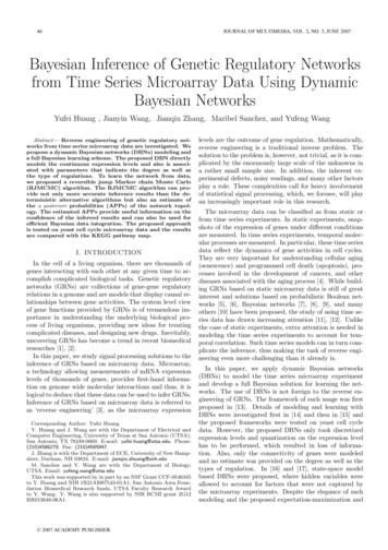
JOURNAL OF MULTIMEDIA, VOL. 2, NO. 3, JUNE 200751period of 119 minutes where a synchronization treatmentbased on α mating factor was used. On the other hand, thedata set from [28] contains 17 samples evenly measured over160 minutes, and a temperature-sensitive cdc15 mutant wasused for synchronization. For each gene, the data is represented as the log2 {(expression at time t)/(expression inmixture of control cells)}. Missing values exist in both datasets, which indicate that there was not a sufficiently strongsignal in the spot. In this case, simple spline interpolationwas used to fill in the missing data.As to the RJMCMC algorithm, in all of the experimentswe used γ0 0.36 and ν0 1.2; we found that, as long asthey are kept small, the results are insensitive to their specific values. Also, when implementing the RJMCMC algorithm, we set T 10, 000 and ran the algorithm 10 timesindependently. In each independent run, we discard thefirst 1000 samples. This resulted in a total of 90,000 samples. By having independent runs, we reduce the chanceof the Markov chains being trapped in local high densityregions, thus lowering the bias of the samples.B. Test on a simulated network-110variance σ 2 of the RJMCMC and K2 algorithms. For bothalgorithms, the POE at a given σ 2 was calculated basedon 100 Monte Carlo trials. For the RJMCMC, we choseQmax 5 and q 2/58. For the K2 algorithm, since noordering was available, we performed an exhaustive searchto determine the first possible parent of the selected gene.Also, the geometric prior on topology was included in theK2 algorithm. Figure 2 clearly demonstrates better performance of the RJMCMC algorithm, especially for smallσ 2 . Notice that the POE of the RJMCMC decreases drastically with σ 2 , whereas the POE of the K2 algorithm almostremains flat for different σ 2 . This suggests that the K2was trapped in some local solutions. The figure also suggests that when σ 2 increases to a point that noise becomesmuch stronger than the information from data, neither algorithm could perform well. However, this case is of littleinterest and more data should be included instead. Theestimated variance from the real data set is 0.52. Giventhe correctness of the model, we would then expect betterperformance of the RJMCMC than the K2 when both wereapplied to the real data set. In summary, through this teston the simulated network, we are assured that the RJMCMC indeed works and has the potential to provide muchbetter results.Probability of errorC. Tests on the real data setsUnconfirmed byKEGG pathway-210Bub1Bub3Dbf4Pho85Up regulateDown cc3Tup1Cln3Cks10.8Swi4Noise variance Swi5We first tested the RJMCMC algorithm on a simulated network and compared the performance with the wellknown K2 algorithm [30]. Since the algorithm was appliedto each gene separately, we thus only tested the performance of the algorithm on a randomly selected gene. Torealistically simulate the network of the selected gene, wefirst ran the RJMCMC algorithm on the real data set fromthe α factor synchronization to estimate the parents, theassociated weights, and the noise variance. Then the results on the parents and the weights were used as the truemodel parameters when simulating the expression level ofthe selected gene for time samples 2 to 18, whereas the expression level of the parent genes were still taken from thereal data set. The resulted data set was then almost thesame as the real data set, except the data of the selectedgene were replaced by the simulated data. In Figure 2,we plotted the probability of errors (POE) vs. the noiseCdc45Clb6Fig. 2. Plot of the probability of error vs. the noise variance for theRJMCMC and the K2 algorithms. 2007 ACADEMY PUBLISHERWeight from 0.8—1.5Mec3Cdc280Weight from 0.4—0.8Bub2Rad2410Weight from Pho80Cak1Met30Esr1Rad9Lte1Fig. 3. The inferred gene network for Qmax 10 and q 6/58.In this section, we provide the test results of RJMCMCon the two real data sets from yeast cell cycles. In thefirst experiment, we set the upper limit on the number ofparents as Qmax 10 and assume that, on average, therewere 6 parents for each gene, which implies q 6/58. Theinferred gene network is depicted in Figure 3. In this network, the nodes are labeled with gene names and, like inDBNs, if gene i is a parent of gene j, an arrow from i to jis placed. The thickness of the arrow is determined by themagnitude of the corresponding weight, which denotes the

52JOURNAL OF MULTIMEDIA, VOL. 2, NO. 3, JUNE D24CD

M. Sanchez and Y. Wang are with the Department of Biology, UTSA. Email: yufeng.wang@utsa.edu This work was supported by in part by an NSF Grant CCF-0546345 to Y. Huang and NIH 1R21AI067543-01A1, San Antonio Area Foun-dation Biomedical Research funds, UTSA Faculty Research Award