WIXLIB

ECE 3530 / CS 3130 Spring 20157she was deeply concerned with issues of discrimination and social justice. Before entering theworkforce, Linda spent time in the Peace Corps helping women gain access to health care in andaround the Congo region of Africa. Which is most likely?1. Linda is a bank teller.2. Linda is a bank teller and writes for a feminism blog.This question is adapted from a question posed to U. of British Columbia undergraduates in1983 by Amos Tversky and Daniel Kahneman. They found 85% of students rated (2) as more likelythan (1). However, if we define A the event that Linda is a bank teller, and B the event thatLinda writes for a feminism blog, then (1) has probability P [A], and (2) has probability P [A B].The laws of probability, as we will see, mandate that P [A B] P [A], with equality only if allbank tellers write for feminism blogs. In short, Tversky and Kahneman noticed that people areswayed by a narrative – the more detail, the more believable it seems.Example: Probability of Failure in DisastersConsider a hypothetical nuclear reactor located near an ocean that will leak radiation only if thereis both a severe earthquake, and simultaneously a flood in the reactor facility. The probability ofan severe earthquake is, on any given day, 1/10,000, and the probability of a flood in the facility is1/5,000. What is the probability the nuclear reactor will leak radiation?There is a tendency, without thinking about the events in question, to assume they are independent, and thus the probability P [A B] P [A] P [B]. In this case would lead to a probability of1, or one in 50 million. That would be, about once every 130,000 years. Based on this analysis,5 107an engineer might say, this facility will never fail. However, it would be more accurate to realizethe events are closely related, that a tsunami can be both a severe earthquake, and cause majorflooding at the same time. The rate of leaks would be close to the probability of a major tsunami,something likely to happen in an average person’s lifetime.In summary, intuition is not a good way to approach problems in probability and statistics. Itis important to follow the methods we will present in this course. It is also important to have lotsof practice – repetition will help to train us on the proper procedure for analysis.Lecture #22Events as SetsAll probability is defined on sets. In probability, we call these sets events. A set is a collection ofelements. In probability, we call these outcomes. The words we use for events is slightly differentthan what you did when you learned sets in a math class, see Table 2.Def ’n: EventA collection of outcomes. Order doesn’t matter, and there are no duplicates.2.1IntroductionThere are different ways to define an event (set):

ECE 3530 / CS 3130 Spring 2015Set Theoryuniverseelementsetdisjoint setsnull set8Probability Theorysample space (certain event)outcome (sample point)eventdisjoint eventsnull eventProbability SymbolSsEE1 E2 Table 1: Set Terminology vs. Probability TerminologySSBAASBAAB(a)(b)B(c)Figure 1: Venn diagrams of sample space S and two sets A and B which (a) are not disjoint, (b)are disjoint, and (c) form a partition of S. List them: A {0, 5, 10, 15, . . .}; B {T ails, Heads}. As an interval: [0, 1], [0, 1), (0, 1), (a, b]. Be careful: the notation overlaps with that forcoordinates! An existing event set name: N, R2 , Rn . By rule: C {x R x 0}, D {(x, y) R2 x2 y 2 R2 }.2.2Venn DiagramsVenn diagrams can be used to pictorially show whether or not there is overlap between two or moresets. They are a good tool for helping remember some of the laws of probability. We don’t usethem in proofs, however, they’re particularly good to develop intuition.2.3Important EventsHere’s an important event: {}, the null event or the empty set.Here’s the opposite: S is used to represent the set of everything possible in a given context, thesample space. S B above for the flip of a coin. S {1, 2, 3, 4, 5, 6} for the roll of a (6-sided) die. S {Adenine, Cytosine, Guanine, T hymine} for the nucleotide found at a particular placein a strand of DNA. S C, i.e., non-negative real numbers, for your driving speed (maybe when the cop pullsyou over).

ECE 3530 / CS 3130 Spring 20152.49Operating on EventsWe can operate on one or more events: Complement: Ac {x S x / A}. We must know the sample space S! Union: A B {x x A or x B}. Merges two events together. Intersection: A B {x x A and x B}. Limits to outcomes common to both events.DO NOT use addition to represent the union, and DO NOT use multiplication to represent theintersection. An example of why this is confusing:{1} {1} {1}.This leads to one of the most common written mistakes – exchanging unions and plusses whencalculating probabilities. Don’t write P [A] P [B] when you really mean P [A B]. Don’t addsets and numbers: for example, if A and B are sets, don’t write P [A] B.2.5Disjoint SetsDef ’n: DisjointTwo events A1 and A2 are disjoint if A1 A2 .Def ’n: Mutually exclusiveMultiple events A1 , A2 , A3 , . . . are mutually exclusive if every pair of events is disjoint.Some disjoint events: {1, 2} and {6}; A and Ac ; A and .3ProbabilityYou’re familiar with functions, like f (x) x2 , which assign a number output to each number input.Probability assigns a number output to each event input.3.1How to Assign Probabilities to EventsAs long as we follow three intuitive rules (axioms) our assignment can be called a probability model.Axiom 1: For any event A, P [A] 0.Axiom 2: P [S] 1.Axiom 3: For any two disjoint events A1 and A2 ,P [A1 A2 ] P [A1 ] P [A2 ] .The final axiom in the Walpole book is more complicated:Axiom 3: If A1 , A2 , A3 , . is a sequence of mutually exclusive events, thenP [A1 A2 A3 · · ·] P [A1 ] P [A2 ] P [A3 ] · · ·

ECE 3530 / CS 3130 Spring 201510However, one may prove the more complicated Walpole Axiom 3 from the three axioms given above.For details, see [Billingsley 1986].Example: DNA MeasurementConsider the DNA experiment above. We measure from a strand of DNA its first nucleotide.Let’s assume that each nucleotide is equally likely. Using axiom 3,P [{a, c, g, t}] P [{a}] P [{c}] P [{g}] P [{t}]But since P [{a, c, g, t}] P [S], by Axiom 2, the LHS is equal to 1. Also, we have assumed thateach nucleotide is equally likely, so1 4P [{a}]So P [{a}] 1/4.Def ’n: Discrete Uniform Probability LawIn general, for event A in a discrete sample space S composed of equally likely outcomes,P [A] 3.2 A S Properties of Probability Models1. P [Ac ] 1 P [A]. Proof:First, note that A Ac S from above. ThusP [A Ac ] P [S]Since A Ac from above, these two events are disjoint.P [A] P [Ac ] P [S]Finally from Axiom 2,P [A] P [Ac ] 1And we have proven what was given.Note that this implies that P [S c ] 1 P [S], and from axiom 2, P [ ] 1 1 0.2. For any events E and F (not necessarily disjoint),P [E F ] P [E] P [F ] P [E F ]Essentially, by adding P [E] P [F ] we double-count the area of overlap. Look at the Venndiagram in Figure 1(a). The P [E F ] term corrects for this. Proof: Do on your own usingthese four steps:(a) Show P [A] P [A B] P [A B c ].(b) Same thing but exchange A and B.(c) Show P [A B] P [A B] P [A B c ] P [Ac B].

ECE 3530 / CS 3130 Spring 201511(d) Combine and cancel.3. Subset rule: If A B, then P [A] P [B]. Proof:Let B (A B) (Ac B). The two events, (A B) and (Ac B), are disjoint sinceA B Ac B . Thus:P [B] P [A B] P [Ac B] P [A] P [Ac B] P [A]Note P [A B] P [A] since A B, and the inequality in the final step is due to the Axiom1.4. Union bound: P [A B] P [A] P [B]. Proof: directly from 2 and Axiom 1.5. Conjunction bound: P [A B] P [A]. Proof: A B is a subset of A. This then followsfrom the subset rule above. See the “Conjunction Fallacy” from lecture 1.Lecture #34Total ProbabilityWe mentioned in passing the very important rule that for any two events A and B,P [A] P [A B] P [A B c ] .(1)This is a simple example of the law of total probability applied to the partition, B and B c . Now,let’s present the more general law of total probability. First, the definition of partition:Def ’n: PartitionSA countable collection of mutually exclusive events C1 , C2 , . . . is a partition if i 1 Ci S.Examples:1. For any set C, the collection C, C c .2. The collection of all simple events for countable sample spaces. Eg., {1}, {2}, {3}, {4}, {5},{6}.Def ’n: Law of Total ProbabilityFor a partition C1 , C2 , . . ., and event A,P [A] P [A C1 ] P [A C2 ] P [A C3 ] · · ·(2)Note: You must use a partition!!!, but A can be any event.Example: Die and OddLet’s consider a fair 6-sided die again, but define the following sets: E1 {1, 2, 3}, E2 {4, 5},and E3 {6}. Also let F be the event that the number rolled is odd. First, find:1. P [Ei F ] for i 1, 2, 3.

ECE 3530 / CS 3130 Spring 2015122. Do E1 , E2 , and E3 form a partition?3. Use (1.) and (2.) to calculate P [F ].Solution:1. Using the discrete uniform probability law, P [E1 F ] 2/6, P [E2 F ] 1/6, and P [E3 F ] 0/6 .2. Well, E1 E2 E3 {1, 2, 3, 4, 5, 6} S and the intersection of any two of the Ei sets is thenull set. So they do form a partition.3. By the law of total probability, P [F ] P [E1 F ] P [E2 F ] P [E3 F ] 2 1 06 0.5.Example: TraitsPeople may inherit genetic trait A or not; similarly, they may inherit genetic trait B or not.People with both traits A and B are at higher risk for heart disease. For the general population,P [A] 0.50, and P [B] 0.10. We know that P [A B c ], that is, the probability of having traitA but not trait B, is 0.48. What is the probability of having both trait A and B?Solution: Use the law of total probability with partition B and B c :P [A] P [A B] P [A B c ] .We can rearrange to: P [A B] P [A] P [A B c ]. Using the given information:P [A B] 0.50 0.48 0.02.A Venn diagram is particularly helpful here.4.1TreesA graphical method for organizing information about how a multiple-stage experiment can occur.See Figure 2.Example: Customers Satisfied by OperatorA tech support phone bank has exactly three employees. A caller is randomly served by one ofthe three. After a customer is served, he or she is surveyed. TData is kept as to the employee (bynumber, 1, 2, or 3) and whether the caller was satisfied (S). The data shows: P [S 1] 0.40 P [S 2] 0.20 P [S 3] 0.18Questions:1. What is the probability that a caller is satisfied?2. Are the probabilities of a caller being served by each of the three employees equal?Solution:

ECE 3530 / CS 3130 Spring 201513Operation #1First option foroperation #1Operation #2First option for operation #2given 1st for op. #1Second option for operation #2given 1st for op. #1First option for operation #2given 2nd for op. #1Second optionfor operation #1Second option for operation #2given 2nd for op. #1Third option for operation #2given 2nd for op. #1Figure 2: A tree shows the options of a first operation, and then for each of those options, whatoptions exist for the second operation. The number of branches at each node does not need to bethe same.1. Since 1, 2, and 3 are a partition, P [S] P [S 1] P [S 2] P [S 3] 0.4 0.2 0.18 0.78.2. The three probabilities, P [1], P [2], and P [3] can’t be equal. Employee 1 has too high ofa probability. By the conjunction bound, P [1] P [S 1] 0.40. Note you can get theconjunction bound by considering thatP [1] P [1 S] P [1 S c ]P [1] P [1 S] .(3)The latter line because the probability P [1 S c ] 0 by probability Axiom 1.In any case, the probability a caller is served by 1 is at least 40%. If the three employees wereequally likely, they’d each have probability of 0.333.Lecture #45CountingThis section covers how to determine the size, i.e., the number of outcomes, in the sample space orin an event.Example: Tablet SpecsA tablet manufactured by Pear Computer Co can have 64 GB, 32 GB, or 16 GB of memory, andcan either have 4G connectivity or not. How many different versions of tablet does Pear make?Solution: The solution is 6: (64, 4G), (64, No), (32, 4G), (32, No), (16, 4G), (16, No).

ECE 3530 / CS 3130 Spring 20155.114Multiplication RuleWhat is the general formula for this, so we don’t have to list outcomes?Def ’n: Multiplication RuleIf one operation can be performed in n1 ways, and for each of those ways, a second operation canbe performed in n2 ways, then there are n1 n2 ways to perform the two operations together.Example: Form EntryA web form asks for 1) a person’s state of birth (or n/a if not born in the US) and 2) a pin codebetween 0 and 9999. How many different entries are possible?Solution: There are 50 states and 1 n/a, for a total of 51 ways to answer the first question, and10,000 ways to answer the second question. By the multiplication rule, there are 51(104 ) 5.1 105different entries possible.We don’t need to stop at two “operations” – many problems involve more.Def ’n: Multiplication RuleIf a first operation can be performed in n1 ways, and for each of those ways, a second operationcan be performed in n2 ways, and for each of those ways to do both operations together, there aren3 ways to do a third operation, and so forth through the kth operation, then there are n1 n2 · · · nkways to perform the k operations together.Example: Phonics testingThe state of Utah tests early elementary students on their ability in phonics by presenting themwith a (potentially fake) three letter word and asking them to pronounce it. The first letter is aconsonant, the second a vowel (excluding y), and the third a consonant. The consonant is allowedto repeat. How many different questions could there be?Solution: There are 26 letters, five of them vowels (a e i o u). Thus there are 21 consonants. Thefirst letter must be one of 21, the second letter must be one of five vowels, and the third letter isone of 21 consonants again. The answer is (21)(5)(21) 2205.Example: Turn in orderThere are 115 students in a class taking an exam. Consider the first, second, and third person toturn in their exam. How many ways can this happen? Assume order is important, and each personcan turn in their exam only once.Solution: The first person can be any of the 115. The second person can’t be the same as the1st, so is one of the remaining 114. The third is similarly one of the remaining 113. Thus there are(115)(114)(113) 1, 481, 430 ways for this order to happen.5.2PermutationsIn general, when we take elements of a set (such as the students in a class, above) and order a few(or all) of them, it is called a permutation.The number of ways to put r elements in order, from a set of n unique possibilities, is denotedPn r , and is calculated as:n Pr n! n · (n 1) · (n 2) · · · (n r 1)(n r)!(4)

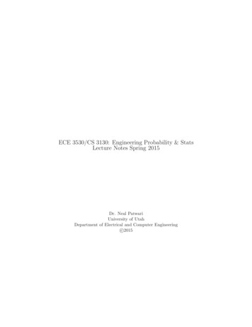
ECE 3530 / CS 3130 Spring 201515Note 0! 1! 1.If you’re going to order ALL of the elements of the set, then r n, so there are n · (n 1) · (n 2) · · · 1 n! ways to order them.Example: Cards in the deckOrder is important in a card deck because it affects which player will get each card.1. How many ways are there to order the 52 cards in a standard card deck?2. How many ways are there to pick 4 cards, in order which you pick them, from a standardcard deck?Example: Three pillsYou are sick and there are three pills in front of you, one which will do nothing (N), one which willkill you (K), and one which will cure you (C). You have no idea which one is which. You will putthe three pills in order, and take one at a time, and stop when you either get cured or killed.1. How many ways are there to put the pills in order from first to last? (You might stop beforeyou get to the end, but just answer how many ways there are to put them in order.2. How many ways are there to order the three pills that will cure you?Lecture #56Counting6.1Birthday Paradox: a Permutation ExampleExample: Birthday ParadoxWhat is the probability that two people in this room will have the same birthday? Assume that“birthday” doesn’t include year, and that each day of the year is equally likely (and exclude theleap day), and that each person’s birthday is independent.Solution:1. How many ways are there for n people to have their birthday? Answer: Each person canhave their birthday happen in one of 365 ways, assuming 365 days per year. So: 365n .2. How many ways are there to have all n people have unique birthdays? The first one canhappen in 365 ways, the second has 364 left, and so on: 365 Pn 365!/(365 n)!.3. Discrete uniform probability law:P [ no duplicate birthdays] 365!/(365 n)!365nSee Fig. 3, which ends at n 30. At n 50, there is only a 3% chance. At n 60, there isa 0.6% chance. At 110 students (our entire class) the probability is on the order of 10 8 . This iscalled the birthday paradox because most people would not guess that it would be so likely to havetwo people with a common birthday in a group as small as 20 or 30.

ECE 3530 / CS 3130 Spring 201516P[ No Repeat Birthdays]10.750.50.25001020Number of People in Group30Figure 3: The probability of having no people with matching birth dates in a group of people, vs.the number in the group. Note the probability is less than half when the class is bigger than 23.6.2CombinationsPermutations require that the order matters. For example, in the three pills example where youtake one pill at a time until you die or are cured, where K is the pill that will kill you, and C is thepill that will cure you, KC is different than CK (as different as life and death!). Certainly in wordsor license plates, as well, the order of the chosen letters matter. However, sometimes order doesn’tmatter, ie, if you are counting how many different sets could exist (since order doesn’t matter in aset). As another example, in many card games you are dealt a hand which you can re-order as youwish, thus the order you were dealt the hand doesn’t matter.Def ’n: CombinationsThe number of (unordered) combinations of size r taken from n distinct objects is n!n. r(n r)!r!We can think of permutations as overcounting in the case when order doesn’t matter. If orderdoesn’t matter and we order r distinct objects from a set of n, we’d count them as n!/(n r)!. Butfor each ordering of length r, somewhere else in the permutation set is a different ordering of thesame r objects. Since there are r! ways to order these r objects, the formula n Pr overcounts thenumber of combinations by a factor of r!, or: 11n!n n Pr .rr!(n r)! r!Example: 5-card PokerHow many ways are there to be dealt a 5-card hand from a standard 52-card deck, where orderdoesn’t matter? Note that in poker, all 52 cards are distinct.Solution: We are taking r 5 cards from a n 52 distinct objects. Thus 52 · 51 · 50 · 49 · 4852!52 2, 598, 960 5(52 5)!5!5·4·3·2·1

ECE 3530 / CS 3130 Spring 201517Example: PokerEvaluate the probabilities of being dealt a “flush” in a five card poker hand. Note the The s

1 Intro to Probability and Statistics 5 . or process may be random, we as engineers are able to ‘measure’ them. For example: The expected value is a tool which tells us, if we observed lots of realizations