Transcription
ComplimentsofDeepLearningA PRACTITIONER'S APPROACHCEEFRSRETPAHJosh Patterson &Adam Gibson
ELIMINATEDATA STORAGEBOTTLENECKSReduce time from data to intelligencewith a modern data platform.Visit purestorage.com/analytics to learn more 2017 Pure Storage, Inc. All rights reserved. Pure Storage and theP logo are trademarks or registered trademarks of Pure Storage, Inc.
Deep LearningA Practitioner’s ApproachThis Excerpt contains Chapters 1 and 3 of the book DeepLearning. The full book is available on oreilly.com andthrough other retailers.Josh Patterson and Adam GibsonBeijingBoston Farnham SebastopolTokyo
Deep Learningby Josh Patterson and Adam GibsonCopyright 2017 Josh Patterson and Adam Gibson. All rights reserved.Printed in the United States of America.Published by O’Reilly Media, Inc., 1005 Gravenstein Highway North, Sebastopol, CA 95472.O’Reilly books may be purchased for educational, business, or sales promotional use. Online editions arealso available for most titles (http://oreilly.com/safari). For more information, contact our corporate/insti‐tutional sales department: 800-998-9938 or corporate@oreilly.com.Editors: Mike Loukides and Tim McGovernProduction Editor: Nicholas AdamsCopyeditor: Bob Russell, Octal Publishing, Inc.Proofreader: Christina EdwardsAugust 2017:Indexer: Judy McConvilleInterior Designer: David FutatoCover Designer: Karen MontgomeryIllustrator: Rebecca DemarestFirst EditionRevision History for the First Edition2017-07-27: First ReleaseSee http://oreilly.com/catalog/errata.csp?isbn 9781491914250 for release details.The O’Reilly logo is a registered trademark of O’Reilly Media, Inc. Deep Learning, the cover image, andrelated trade dress are trademarks of O’Reilly Media, Inc.While the publisher and the authors have used good faith efforts to ensure that the information andinstructions contained in this work are accurate, the publisher and the authors disclaim all responsibilityfor errors or omissions, including without limitation responsibility for damages resulting from the use ofor reliance on this work. Use of the information and instructions contained in this work is at your ownrisk. If any code samples or other technology this work contains or describes is subject to open sourcelicenses or the intellectual property rights of others, it is your responsibility to ensure that your usethereof complies with such licenses and/or rights.978-1-492-02379-1[LSI]
Table of Contents1. A Review of Machine Learning. . . . . . . . . . . . . . . . . . . . . . . . . . . . . . . . . . . . . . . . . . . . . . . . . 1The Learning MachinesHow Can Machines Learn?Biological InspirationWhat Is Deep Learning?Going Down the Rabbit HoleFraming the QuestionsThe Math Behind Machine Learning: Linear evant Mathematical OperationsConverting Data Into VectorsSolving Systems of EquationsThe Math Behind Machine Learning: StatisticsProbabilityConditional ProbabilitiesPosterior ProbabilityDistributionsSamples Versus PopulationResampling MethodsSelection BiasLikelihoodHow Does Machine Learning 151618191922222223232325iii
ClusteringUnderfitting and OverfittingOptimizationConvex OptimizationGradient DescentStochastic Gradient DescentQuasi-Newton Optimization MethodsGenerative Versus Discriminative ModelsLogistic RegressionThe Logistic FunctionUnderstanding Logistic Regression OutputEvaluating ModelsThe Confusion MatrixBuilding an Understanding of Machine Learning26262729303233333435353636402. Fundamentals of Deep Networks. . . . . . . . . . . . . . . . . . . . . . . . . . . . . . . . . . . . . . . . . . . . . 41Defining Deep LearningWhat Is Deep Learning?Organization of This ChapterCommon Architectural Principles of Deep NetworksParametersLayersActivation FunctionsLoss FunctionsOptimization AlgorithmsHyperparametersSummaryBuilding Blocks of Deep NetworksRBMsAutoencodersVariational Autoencodersiv Table of Contents414151525253535556606565667274
CHAPTER 1A Review of Machine LearningTo condense fact from the vapor of nuance—Neal Stephenson, Snow CrashThe Learning MachinesInterest in machine learning has exploded over the past decade. You see machinelearning in computer science programs, industry conferences, and the Wall StreetJournal almost daily. For all the talk about machine learning, many conflate what itcan do with what they wish it could do. Fundamentally, machine learning is usingalgorithms to extract information from raw data and represent it in some type ofmodel. We use this model to infer things about other data we have not yet modeled.Neural networks are one type of model for machine learning; they have been aroundfor at least 50 years. The fundamental unit of a neural network is a node, which isloosely based on the biological neuron in the mammalian brain. The connectionsbetween neurons are also modeled on biological brains, as is the way these connec‐tions develop over time (with “training”). We’ll dig deeper into how these modelswork over the next two chapters.In the mid-1980s and early 1990s, many important architectural advancements weremade in neural networks. However, the amount of time and data needed to get goodresults slowed adoption, and thus interest cooled. In the early 2000s computationalpower expanded exponentially and the industry saw a “Cambrian explosion” of com‐putational techniques that were not possible prior to this. Deep learning emergedfrom that decade’s explosive computational growth as a serious contender in the field,winning many important machine learning competitions. The interest has not cooledas of 2017; today, we see deep learning mentioned in every corner of machinelearning.1
We’ll discuss our definition of deep learning in more depth in the section that follows.This book is structured such that you, the practitioner, can pick it up off the shelf anddo the following: Review the relevant basic parts of linear algebra and machine learningReview the basics of neural networksStudy the four major architectures of deep networksUse the examples in the book to try out variations of practical deep networksWe hope that you will find the material practical and approachable. Let’s kick off thebook with a quick primer on what machine learning is about and some of the coreconcepts you will need to better understand the rest of the book.How Can Machines Learn?To define how machines can learn, we need to define what we mean by “learning.” Ineveryday parlance, when we say learning, we mean something like “gaining knowl‐edge by studying, experience, or being taught.” Sharpening our focus a bit, we canthink of machine learning as using algorithms for acquiring structural descriptionsfrom data examples. A computer learns something about the structures that representthe information in the raw data. Structural descriptions are another term for themodels we build to contain the information extracted from the raw data, and we canuse those structures or models to predict unknown data. Structural descriptions (ormodels) can take many forms, including the following: Decision trees Linear regression Neural network weightsEach model type has a different way of applying rules to known data to predictunknown data. Decision trees create a set of rules in the form of a tree structure andlinear models create a set of parameters to represent the input data.Neural networks have what is called a parameter vector representing the weights onthe connections between the nodes in the network. We’ll describe the details of thistype of model later on in this chapter.2 Chapter 1: A Review of Machine Learning
Machine Learning Versus Data MiningData mining has been around for many decades, and like many terms in machinelearning, it is misunderstood or used poorly. For the context of this book, we considerthe practice of “data mining” to be “extracting information from data.” Machine learn‐ing differs in that it refers to the algorithms used during data mining for acquiring thestructural descriptions from the raw data. Here’s a simple way to think of data mining: To learn concepts— we need examples of raw data Examples are made of rows or instances of the data— Which show specific patterns in the data The machine learns concepts from these patterns in the data— Through algorithms in machine learningOverall, this process can be considered “data mining.”Arthur Samuel, a pioneer in artificial intelligence (AI) at IBM and Stanford, definedmachine learning as follows:[The f]ield of study that gives computers the ability to learn without being explicitlyprogrammed.Samuel created software that could play checkers and adapt its strategy as it learnedto associate the probability of winning and losing with certain dispositions of theboard. That fundamental schema of searching for patterns that lead to victory ordefeat and then recognizing and reinforcing successful patterns underpins machinelearning and AI to this day.The concept of machines that can learn to achieve goals on their own has captivatedus for decades. This was perhaps best expressed by the modern grandfathers of AI,Stuart Russell and Peter Norvig, in their book Artificial Intelligence: A ModernApproach:How is it possible for a slow, tiny brain, whether biological or electronic, to perceive,understand, predict, and manipulate a world far larger and more complicated thanitself?This quote alludes to ideas around how the concepts of learning were inspired fromprocesses and algorithms discovered in nature. To set deep learning in context visu‐ally, Figure 1-1 illustrates our conception of the relationship between AI, machinelearning, and deep learning.The Learning Machines 3
Figure 1-1. The relationship between AI and deep learningThe field of AI is broad and has been around for a long time. Deep learning is a sub‐set of the field of machine learning, which is a subfield of AI. Let’s now take a quicklook at another of the roots of deep learning: how neural networks are inspired bybiology.Biological InspirationBiological neural networks (brains) are composed of roughly 86 billion neurons con‐nected to many other neurons.Total Connections in the Human BrainResearchers conservatively estimate there are more than 500 tril‐lion connections between neurons in the human brain. Even thelargest artificial neural networks today don’t even come close toapproaching this number.4 Chapter 1: A Review of Machine Learning
From an information processing point of view a biological neuron is an excitable unitthat can process and transmit information via electrical and chemical signals. A neu‐ron in the biological brain is considered a main component of the brain, spinal cordof the central nervous system, and the ganglia of the peripheral nervous system. Aswe’ll see later in this chapter, artificial neural networks are far simpler in their compa‐rative structure.Comparing Biological with ArtificialBiological neural networks are considerably more complex (severalorders of magnitude) than the artificial neural network versions!There are two main properties of artificial neural networks that follow the generalidea of how the brain works. First is that the most basic unit of the neural network isthe artificial neuron (or node in shorthand). Artificial neurons are modeled on thebiological neurons of the brain, and like biological neurons, they are stimulated byinputs. These artificial neurons pass on some—but not all—information they receiveto other artificial neurons, often with transformations. As we progress through thischapter, we’ll go into detail about what these transformations are in the context ofneural networks.Second, much as the neurons in the brain can be trained to pass forward only signalsthat are useful in achieving the larger goals of the brain, we can train the neurons of aneural network to pass along only useful signals. As we move through this chapterwe’ll build on these ideas and see how artificial neural networks are able to modeltheir biological counterparts through bits and functions.Biological Inspiration Across Computer ScienceBiological inspiration is not limited to artificial neural networks in computer science.Over the past 50 years, academic research has explored other topics in nature forcomputational inspiration, such as the following: AntsTermites1BeesGenetic algorithmsAnt colonies, for instance, have been by researchers to be a powerful decentralizedcomputer in which no single ant is a central point of failure. Ants constantly switch1 Patterson. 2008. “TinyTermite: A Secure Routing Algorithm” and Sartipi and Patterson. 2009. “TinyTermite: ASecure Routing Algorithm on Intel Mote 2 Sensor Network Platform.”The Learning Machines 5
tasks to find near optimal solutions for load balancing through meta-heuristics suchas quantitative stigmergy. Ant colonies are able to perform midden tasks, defense,nest construction, and forage for food while maintaining a near-optimal number ofworkers on each task based on the relative need with no individual ant directly coor‐dinating the work.What Is Deep Learning?Deep learning has been a challenge to define for many because it has changed formsslowly over the past decade. One useful definition specifies that deep learning dealswith a “neural network with more than two layers.” The problematic aspect to thisdefinition is that it makes deep learning sound as if it has been around since the1980s. We feel that neural networks had to transcend architecturally from the earliernetwork styles (in conjunction with a lot more processing power) before showing thespectacular results seen in more recent years. Following are some of the facets in thisevolution of neural networks: More neurons than previous networksMore complex ways of connecting layers/neurons in NNsExplosion in the amount of computing power available to trainAutomatic feature extractionFor the purposes of this book, we’ll define deep learning as neural networks with alarge number of parameters and layers in one of four fundamental network architec‐tures: Unsupervised pretrained networksConvolutional neural networksRecurrent neural networksRecursive neural networksThere are some variations of the aforementioned architectures—a hybrid convolu‐tional and recurrent neural network, for example–as well. For the purpose of thisbook, we’ll consider the four listed architectures as our focus.Automatic feature extraction is another one of the great advantages that deep learninghas over traditional machine learning algorithms. By feature extraction, we mean thatthe network’s process of deciding which characteristics of a dataset can be used asindicators to label that data reliably. Historically, machine learning practitioners havespent months, years, and sometimes decades of their lives manually creating exhaus‐tive feature sets for the classification of data. At the time of deep learning’s Big Bangbeginning in 2006, state-of-the-art machine learning algorithms had absorbed deca‐des of human effort as they accumulated relevant features by which to classify input.Deep learning has surpassed those conventional algorithms in accuracy for almost6 Chapter 1: A Review of Machine Learning
every data type with minimal tuning and human effort. These deep networks canhelp data science teams save their blood, sweat, and tears for more meaningful tasks.Going Down the Rabbit HoleDeep learning has penetrated the computer science consciousness beyond most tech‐niques in recent history. This is in part due to how it has shown not only top-flightaccuracy in machine learning modeling, but also demonstrated generative mechanicsthat fascinate even the noncomputer scientist. One example of this would be the artgeneration demonstrations for which a deep network was trained on a particularfamous painter’s works, and the network was able to render other photographs in thepainter’s unique style, as demonstrated in Figure 1-2.Figure 1-2. Stylized images by Gatys et al., 20152This begins to enter into many philosophical discussions, such as, “can machines becreative?” and then “what is creativity?” We’ll leave those questions for you to ponderat a later time. Machine learning has evolved over the years, like the seasons change:subtle but steady until you wake up one day and a machine has become a championon Jeopardy or beat a Go Grand Master.Can machines be intelligent and take on human-level intelligence? What is AI andhow powerful could it become? These questions have yet to be answered and will not2 Gatys et. al, 2015. “A Neural Algorithm of Artistic Style.”The Learning Machines 7
be completely answered in this book. We simply seek to illustrate some of the shardsof machine intelligence with which we can imbue our environment today through thepractice of deep learning.For an Extended Discussion on AIIf you would like to read more about AI, take a look at Appendix A.Framing the QuestionsThe basics of applying machine learning are best understood by asking the correctquestions to begin with. Here’s what we need to define: What is the input data from which we want to extract information (model)? What kind of model is most appropriate for this data? What kind of answer would we like to elicit from new data based on this model?If we can answer these three questions, we can set up a machine learning workflowthat will build our model and produce our desired answers. To better support thisworkflow, let’s review some of the core concepts we need to be aware of to practicemachine learning. Later, we’ll come back to how these come together in machinelearning and then use that information to better inform our understanding of bothneural networks and deep learning.The Math Behind Machine Learning: Linear AlgebraLinear algebra is the bedrock of machine learning and deep learning. Linear algebraprovides us with the mathematical underpinnings to solve the equations we use tobuild models.A great primer on linear algebra is James E. Gentle’s Matrix Alge‐bra: Theory, Computations, and Applications in Statistics.Let’s take a look at some core concepts from this field before we move on startingwith the basic concept called a scalar.8 Chapter 1: A Review of Machine Learning
ScalarsIn mathematics, when the term scalar is mentioned, we are concerned with elementsin a vector. A scalar is a real number and an element of a field used to define a vectorspace.In computing, the term scalar is synonymous with the term variable and is a storagelocation paired with a symbolic name. This storage location holds an unknown quan‐tity of information called a value.VectorsFor our use, we define a vector as follows:For a positive integer n, a vector is an n-tuple, ordered (multi)set or array of n numbers,called elements or scalars.What we’re saying is that we want to create a data structure called a vector via a pro‐cess called vectorization. The number of elements in the vector is called the “order”(or “length”) of the vector. Vectors also can represent points in n-dimensional space.In the spatial sense, the Euclidean distance from the origin to the point representedby the vector gives us the “length” of the vector.In mathematical texts, we often see vectors written as follows:x1x2x x3.xnOr:x x1, x2, x3, . . . , xnThere are many different ways to handle the vectorization, and you can apply manypreprocessing steps, giving us different grades of effectiveness on the output models.We cover more on the topic of converting raw data into vectors later in this chapterand then more fully in Chapter 5.The Math Behind Machine Learning: Linear Algebra 9
MatricesConsider a matrix to be a group of vectors that all have the same dimension (numberof columns). In this way a matrix is a two-dimensional array for which we have rowsand columns.If our matrix is said to be an n m matrix, it has n rows and m columns.Figure 1-3 shows a 3 3 matrix illustrating the dimensions of a matrix. Matrices are acore structure in linear algebra and machine learning, as we’ll show as we progressthrough this chapter.Figure 1-3. A 3 x 3 matrixTensorsA tensor is a multidimensional array at the most fundamental level. It is a more gen‐eral mathematical structure than a vector. We can look at a vector as simply a subclassof tensors.With tensors, the rows extend along the y-axis and the columns along the x-axis.Each axis is a dimension, and tensors have additional dimensions. Tensors also have arank. Comparatively, a scalar is of rank 0 and a vector is rank 1. We also see that amatrix is rank 2. Any entity of rank 3 and above is considered a tensor.HyperplanesAnother linear algebra object you should be aware of is the hyperplane. In the field ofgeometry, the hyperplane is a subspace of one dimension less than its ambient space.In a three-dimensional space, the hyperplanes would have two dimensions. In twodimensional space we consider a one-dimensional line to be a hyperplane.A hyperplane is a mathematical construct that divides an n-dimensional space intoseparate “parts” and therefore is useful in applications like classification. Optimizingthe parameters of the hyperplane is a core concept in linear modeling, as you’ll seefurther on in this chapter.10 Chapter 1: A Review of Machine Learning
Relevant Mathematical OperationsIn this section, we briefly review common linear algebra operations you should know.Dot productA core linear algebra operation we see often in machine learning is the dot product.The dot product is sometimes called the “scalar product” or “inner product." The dotproduct takes two vectors of the same length and returns a single number. This isdone by matching up the entries in the two vectors, multiplying them, and then sum‐ming up the products thus obtained. Without getting too mathematical (immedi‐ately), it is important to mention that this single number encodes a lot of information.To begin with, the dot product is a measure of how big the individual elements are ineach vector. Two vectors with rather large values can give rather large results, and twovectors with rather small values can give rather small values. When the relative valuesof these vectors are accounted for mathematically with something called normaliza‐tion, the dot product is a measure of how similar these vectors are. This mathematicalnotion of a dot product of two normalized vectors is called the cosine similarity.Element-wise productAnother common linear algebra operation we see in practice is the element-wise prod‐uct (or the “Hadamard product”). This operation takes two vectors of the same lengthand produces a vector of the same length with each corresponding element multi‐plied together from the two source vectors.Outer productThis is known as the “tensor product” of two input vectors. We take each element of acolumn vector and multiply it by all of the elements in a row vector creating a newrow in the resultant matrix.Converting Data Into VectorsIn the course of working in machine learning and data science we need to analyze alltypes of data. A key requirement is being able to take each data type and represent itas a vector. In machine learning we use many types of data (e.g., text, time-series,audio, images, and video).So, why can’t we just feed raw data to our learning algorithm and let it handle every‐thing? The issue is that machine learning is based on linear algebra and solving sets ofequations. These equations expect floating-point numbers as input so we need a wayto translate the raw data into sets of floating-point numbers. We’ll connect these con‐cepts together in the next section on solving these sets of equations. An example ofraw data would be the canonical iris dataset:The Math Behind Machine Learning: Linear Algebra 11
3.0,5.9,2.1,Iris-virginicaAnother example might be a raw text document:Go, Dogs. Go!Go on skatesor go by bike.Both cases involve raw data of different types, yet both need some level of vectoriza‐tion to be of the form we need to do machine learning. At some point, we want ourinput data to be in the form of a matrix but we can convert the data to intermediaterepresentations (e.g., “svmlight” file format, shown in the code example that fol‐lows). We want our machine learning algorithm’s input data to look more like theserialized sparse vector format svmlight, as shown in the following example:1.0 1:0.7500000000000001 2:0.41666666666666663 3:0.702127659574468 4:0.56521739130434792.0 1:0.6666666666666666 2:0.5 3:0.9148936170212765 4:0.69565217391304362.0 1:0.45833333333333326 2:0.3333333333333336 3:0.8085106382978723 4:0.73913043478260880.0 1:0.1666666666666665 2:1.0 3:0.0212765957446808232.0 1:1.0 2:0.5833333333333334 3:0.9787234042553192 4:0.82608695652173921.0 1:0.3333333333333333 3:0.574468085106383 4:0.478260869565217461.0 1:0.7083333333333336 2:0.7500000000000002 3:0.6808510638297872 4:0.56521739130434791.0 1:0.916666666666667 2:0.6666666666666667 3:0.7659574468085107 4:0.56521739130434790.0 1:0.08333333333333343 2:0.5833333333333334 3:0.0212765957446808232.0 1:0.6666666666666666 2:0.8333333333333333 3:1.0 4:1.01.0 1:0.9583333333333335 2:0.7500000000000002 3:0.723404255319149 4:0.52173913043478260.0 2:0.7500000000000002This format can quickly be read into a matrix and a column vector for the labels (thefirst number in each row in the preceding example). The rest of the indexed numbersin the row are inserted into the proper slot in the matrix as “features” at runtime toget ready for various linear algebra operations during the machine learning process.We’ll discuss the process of vectorization in more detail in Chapter 8.12 Chapter 1: A Review of Machine Learning
Here’s a very common question: “why do machine learning algorithms want the datarepresented (typically) as a (sparse) matrix?” To understand that, let’s make a quickdetour into the basics of solving systems of equations.Solving Systems of EquationsIn the world of linear algebra, we are interested in solving systems of linear equationsof the form:Ax bwhere A is a matrix of our set of input row vectors and b is the column vector oflabels for each vector in the A matrix. If we take the first three rows of serializedsparse output from the previous example and place the values in its linear algebraform, it looks like this:Column 1Column 2Column 3Column 40.75000000000000010.41666666666666663 0434790.9148936170212765 0.69565217391304360.45833333333333326 0.33333333333333360.8085106382978723 0.7391304347826088This matrix of numbers is our A variable in our equation, and each independentvalue or value in each row is considered a feature of our input data.What Is a Feature?A feature in machine learning is any column value in the input matrix A that we’reusing as an independent variable. Features can be taken straight from the source data,but most of the time we’re going to use some sort of transformation to get the rawinput data into a form that is more appropriate for modeling.An example would be a column of input that has four different text labels in thesource data. We’d need to scan all of the input data and index the labels being used.We’d then need to normalize these values (0, 1, 2, 3) between 0.0 and 1.0 based oneach label’s index for every row’s column value. These types of transforms greatly helpmachine learning find better solutions to modeling problems. We’ll see more techni‐ques for vectorization transforms in Chapter 5.We want to find coefficients for each column in a given row for a predictor functionthat give us the output b, or the label for each row. The labels from the serializedsparse vectors we looked at earlier would be as follows:The Math Behind Machine Learning: Linear Algebra 13
Labels1.02.02.0The coefficients mentioned earlier become the x column vector (also called theparameter vector) shown in Figure 1-4.Figure 1-4. Visualizing the equation Ax bThis system is said to be “consistent” if there exists a parameter vector x such that thesolution to this equation can be directly written as follows:x A 1bIt’s important to delineate the expression x A-1b from the method of actually com‐puting the solution. This expression only represents the solution itself. The variableA-1 is the matrix A inverted and is computed through a process called matrix inver‐sion. Given that not all matrices can be inverted, we’d like a method to solve this equa‐tion that does not involve matrix inversion. One method is called matrixdecomposition. An example of matrix decomposition in solving systems of linearequations is using lower upper (LU) decomposition to solve for the matrix A. Beyondmatrix decomposition, let’s take a look at the general methods for solving sets of lin‐ear equations.Methods for solving systems of linear equationsThere are two general methods for solving a system of linear equations. The first iscalled the “direct method,” in which we know algorithmically that there are a fixednumber of computations. The other approach is a class of methods known as iterativemethods, in which through a series of approximations and a set of termination condi‐tions we can derive the parameter vector x. The direct class of methods is particularlyeffective when we can fit all of the training data (A and b) in memory on a singlecomputer. Well-known examples of the direct method of solving sets of linear equa‐tions are Gaussian Elimination and the Normal Equations.14 Chapter 1: A Review of Machine Learning
Iterative methodsThe iterative class of methods is particularly effective when our data doesn’t fit intothe main memory on a single computer, and looping t
Published by O’Reilly Media, Inc., 1005 Gravenstein Highway North, Sebastopol, CA 95472. O’Reilly