WIXLIB

LINEAR PROGRAMMING:AN ALGEBRAIC APPROACHWeek 7

The Simplex MethodThe method of corners is not suitable for solving linear programmingproblems when the number of variables or constraints is large. Itsmajor shortcoming is that a knowledge of all the corner points of thefeasible set S associated with the problem is required.Thus we need to reduce the number of points to be inspected. Onetechnique is the simplex method, which was developed in the late1940s by George Dantzig and is based on the Gauss–Jordan eliminationmethod.The simplex method is readily adaptable to the computer, which makesit suitable for solving linear programming problems involving largenumbers of variables and constraints.

An Iterative MethodThe simplex method is an iterative procedure: it is repeatedover and over again.Beginning at some initial feasible solution (a corner point ofthe feasible set S, usually the origin), each iteration brings usto another corner point of S, usually with an improved (butcertainly no worse) value of the objective function.The iteration is terminated when the optimal solution isreached (if it exists).

4.1 The Simplex Method:Standard Maximization Problems

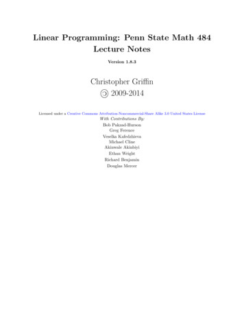
A Standard Maximization ProblemA standard maximization problem is one in which1. The objective function is to be maximized.2. All the variables involved in the problem are nonnegative.3. All other linear constraints may be written so that the expression involving the variablesis less than or equal to a nonnegative constant.Example.Maximizesubject to𝑃 3𝑥 2𝑦2𝑥 3𝑦 122𝑥 𝑦 8𝑥 0, 𝑦 0The optimal solution to the problem occurs at the corner point C(3, 2).

Using the Simplex MethodFirst replace the system of inequality constraints with a system of equality constraints.2𝑥 3𝑦 12 is converted into the equation 2𝑥 3𝑦 𝑢 12The variable 𝑢 is called a slack variable.2𝑥 𝑦8 is converted into the equation 2𝑥 𝑦 𝑣 8Finally, rewriting the objective function in the form 3𝑥 2𝑦 𝑃 0.We are led to the following system of linear equations:2𝑥 3𝑦 𝑢 122𝑥 𝑦 𝑣 8 3𝑥 2𝑦 𝑃 0From among all the solutions of the system for which 𝑥, 𝑦, 𝑢, and 𝑣 are nonnegative (suchsolutions are called feasible solutions), determine the solution(s) that maximizes 𝑃.

The Augmented MatrixObserve that each of the 𝑢-, 𝑣-, and 𝑃-columns of the above augmented matrix is a unitcolumn. The variables associated with unit columns are called basic variables; all othervariables are called non-basic variables.The configuration of the augmented matrix suggests that we solve for the basic variables u,v, and P in terms of the non-basic variables x and y, obtaining𝑢 12 2𝑥 3𝑦𝑣 8 2𝑥 𝑦𝑃 3𝑥 2𝑦

Basic SolutionA particular solution is obtained by letting 𝑥 0 and 𝑦 0.In fact, this solution is given by 𝑥 0, 𝑦 0, 𝑢 12, 𝑣 8, 𝑃 0.Such a solution, obtained by setting the non-basic variables equalto zero, is called a basic solution of the system.This particular solution corresponds to the corner point 𝐴(0, 0) ofthe feasible set associated with the linear programming problem.If the value of 𝑃 cannot be increased, we have found the optimalsolution to the problem at hand.Continuing our quest for an optimal solution, our next task is todetermine whether it is more profitable to increase the value of 𝑥or that of 𝑦 (increasing 𝑥 and 𝑦 simultaneously is more difficult).Is it better to hold 𝑥 0 or 𝑦 0?

How Much Can 𝑥 be IncreasedWhile Holding y 0?Setting 𝑦 0,𝑢 12 2𝑥𝑣 8 2𝑥The first equation and the nonnegativity of 𝑢 imply that x cannot exceed 12/2 or 6.The second equation and the nonnegativity of 𝑣 imply that 𝑥 cannot exceed 8/2 or 4.Thus, we conclude that 𝑥 can be increased by at most 4.Now, if we set 𝑦 0 and 𝑥 4, we obtain the solution𝑥 4, 𝑦 0, 𝑢 4, 𝑣 0, 𝑃 12which is a basic solution to system, this time with 𝑦 and 𝑣 as non-basic variables.We have to find an augmented matrix that has a configuration in which the 𝑥-column is in0the unit form 1 .0

Pivot1. Select the pivot column: Locate the most negative entry to the left of thevertical line in the last row. The column containing this entry is the pivotcolumn. (If there is more than one such column, choose any one.)2. Select the pivot row: Divide each positive entry in the pivot column into itscorresponding entry in the column of constants. The pivot row is the rowcorresponding to the smallest ratio thus obtained. (If there is more than onesuch entry, choose any one.)3. The pivot element is the element common to both the pivot column and thepivot row.

ContinuingConsider the pivot column, use row operations to change the pivot element into 1and non-pivot elements into 0s.Continue to find the next pivot column, pivot row, and pivot element with similarprocedure as before.Then, again, change the pivot element into 1 and non-pivot elements into 0s.We stop the iteration when there are no negative entries in the last row, whichmeans the solution is optimal and 𝑃 cannot be increased further.

Simplex Method First Step:Set Up Initial Simplex Tableu1. Transform the system of linear inequalities into a system of linearequations by introducing slack variables.2. Rewrite the objective function 𝑃 where all the variables are on theleft and the coefficient of 𝑃 is 1.3. Write the tableau associated with this system of linear equations.

ExampleSet up the initial simplex tableau for the linear programming problemMaximize 𝑃 𝑥 1.2𝑦subject to 2𝑥 𝑦 180𝑥 3𝑦 300𝑥 0, 𝑦 0

The Simplex Method1. Set up the initial simplex tableau.2. Determine whether the optimal solution has been reached by examining allentries in the last row to the left of the vertical line.a. If all the entries are nonnegative, the optimal solution has been reached. Proceed to Step 4.b. If there are one or more negative entries, the optimal solution has not been reached.Proceed to Step 3.3. Perform the pivot operation. Locate the pivot element and convert it to a 1 bydividing all the elements in the pivot row by the pivot element. Using rowoperations, convert the pivot column into a unit column by adding suitablemultiples of the pivot row to each of the other rows as required. Return to Step2.4. Determine the optimal solution(s). The value of the variable heading each unitcolumn is given by the entry lying in the column of constants in the rowcontaining the 1. The variables heading columns not in unit form are assignedthe value zero.

ExampleMaximizesubject to𝑃 2𝑥 2𝑦 𝑧2𝑥 𝑦 2𝑧 142𝑥 4𝑦 𝑧 26𝑥 2𝑦 3𝑧 28𝑥 0, 𝑦 0, 𝑧 0

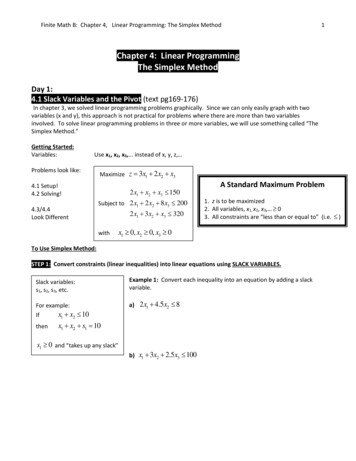
Applied ExampleProduction Planning Ace Novelty Company has determined that the profitfor each Type A, Type B, and Type C souvenir that it plans to produce is 6, 5, and 4, respectively.To manufacture a Type A souvenir requires 2 minutes on Machine I, 1 minuteon Machine II, and 2 minutes on Machine III. A Type B souvenir requires 1minute on Machine I, 3 minutes on Machine II, and 1 minute on Machine III.A Type C souvenir requires 1 minute on Machine I and 2 minutes on each ofMachines II and III.Each day, there are 3 hours available on Machine I, 5 hours available onMachine II, and 4 hours available on Machine III for manufacturing thesesouvenirs.How many souvenirs of each type should Ace Novelty make per day tomaximize its profit?

Problems with Multiple Solutions andProblems with No SolutionsA linear programming problem will have infinitely many solutions if and onlyif the last row to the left of the vertical line of the final simplex tableau has azero in a column that is not a unit column.A linear programming problem will have no solution if the simplex methodbreaks down at some stage.For example, if at some stage there are no nonnegative ratios in ourcomputation, then the linear programming problem has no solution.Example.Maximize𝑃 3𝑥 2𝑦subject to𝑥 𝑦 3𝑥 2𝑥 0, 𝑦 0

4.2 The Simplex Method:Standard Minimization Problems

Minimization with ConstraintsBy changing the problem to a standard maximization problem which satisfies three conditions:1. The objective function is to be maximized.2. All the variables involved are nonnegative.3. Each linear constraint may be written so that the expression involving the variables is less thanor equal to a nonnegative constant.Example.Minimizesubject to𝐶 2𝑥 3𝑦5𝑥 4𝑦 32𝑥 2𝑦 10𝑥 0, 𝑦 0Minimizing the objective function 𝐶 is equivalent to maximizing the objective function 𝑃 𝐶.Maximize 𝑃 2𝑥 3𝑦 subject to the given constraints.

05.03.2020 · Problems with Multiple Solutions and Problems with No Solutions A linear programming problem will have infinitely many solutions if and only if the last row to the left of the vertical line of the final simplex tableau has a zero in a column that is not a unit column. A linear programming problem will have no solution if the simplex method