Transcription
Linear Programming: Theory and ApplicationsCatherine LewisMay 11, 20081
Contents1 Introduction to Linear Programming1.1 What is a linear program? . . . . . . . . . . . . . . . . . . . . . .331.21.3Assumptions . . . . . . . . . . . . . . . . . . . . . . . . . . . . .Manipulating a Linear Programming Problem . . . . . . . . . . .561.41.5The Linear Algebra of Linear Programming . . . . . . . . . . . .Convex Sets and Directions . . . . . . . . . . . . . . . . . . . . .782 Examples from Bazaraa et. al. and Winston112.1 Examples . . . . . . . . . . . . . . . . . . . . . . . . . . . . . . . 112.2Discussion . . . . . . . . . . . . . . . . . . . . . . . . . . . . . . .3 The Theory Behind Linear Programming16173.1Definitions . . . . . . . . . . . . . . . . . . . . . . . . . . . . . . .173.2The General Representation Theorem . . . . . . . . . . . . . . .194 An Outline of the Proof205 Examples With Convex Sets and Extreme Points From Bazaaraet. al.226 Tools for Solving Linear Programs236.1 Important Precursors to the Simplex Method . . . . . . . . . . . 237 The Simplex Method In Practice258 What if there is no initial basis in the Simplex tableau?288.18.2The Two-Phase Method . . . . . . . . . . . . . . . . . . . . . . .The Big-M Method . . . . . . . . . . . . . . . . . . . . . . . . . .29319 Cycling339.1 The Lexicographic Method . . . . . . . . . . . . . . . . . . . . . 349.2Bland’s Rule . . . . . . . . . . . . . . . . . . . . . . . . . . . . .379.39.4Theorem from [2] . . . . . . . . . . . . . . . . . . . . . . . . . . .Which Rule to Use? . . . . . . . . . . . . . . . . . . . . . . . . .373910 Sensitivity Analysis3910.1 An Example . . . . . . . . . . . . . . . . . . . . . . . . . . . . . . 3910.1.1 Sensitivity Analysis for a cost coefficient . . . . . . . . . .140
10.1.2 Sensitivity Analysis for a right-hand-side value . . . . . .4111 Case Study: Busing Children to School4111.1 The Problem . . . . . . . . . . . . . . . . . . . . . . . . . . . . . 4211.2 The Solution . . . . . . . . . . . . . . . . . . . . . . . . . . . . .11.2.1 Variables . . . . . . . . . . . . . . . . . . . . . . . . . . .424211.2.2 Objective Function . . . . . . . . . . . . . . . . . . . . . .11.2.3 Constraints . . . . . . . . . . . . . . . . . . . . . . . . . .434311.3 The Complete Program . . . . . . . . . . . . . . . . . . . . . . .11.4 Road Construction and Portables . . . . . . . . . . . . . . . . . .474911.4.1 Construction . . . . . . . . . . . . . . . . . . . . . . . . .11.4.2 Portable Classrooms . . . . . . . . . . . . . . . . . . . . .495011.5 Keeping Neighborhoods Together . . . . . . . . . . . . . . . . . .11.6 The Case Revisited . . . . . . . . . . . . . . . . . . . . . . . . . .555611.6.1 Shadow Prices . . . . . . . . . . . . . . . . . . . . . . . .5611.6.2 The New Result . . . . . . . . . . . . . . . . . . . . . . .5712 Conclusion572
1Introduction to Linear ProgrammingLinear programming was developed during World War II, when a system withwhich to maximize the efficiency of resources was of utmost importance. Newwar-related projects demanded attention and spread resources thin. “Programming” was a military term that referred to activities such as planning schedulesefficiently or deploying men optimally. George Dantzig, a member of the U.S.Air Force, developed the Simplex method of optimization in 1947 in order toprovide an efficient algorithm for solving programming problems that had linearstructures. Since then, experts from a variety of fields, especially mathematicsand economics, have developed the theory behind “linear programming” andexplored its applications [1].This paper will cover the main concepts in linear programming, includingexamples when appropriate. First, in Section 1 we will explore simple properties, basic definitions and theories of linear programs. In order to illustratesome applications of linear programming, we will explain simplified “real-world”examples in Section 2. Section 3 presents more definitions, concluding with thestatement of the General Representation Theorem (GRT). In Section 4, we explore an outline of the proof of the GRT and in Section 5 we work through afew examples related to the GRT.After learning the theory behind linear programs, we will focus methodsof solving them. Section 6 introduces concepts necessary for introducing theSimplex algorithm, which we explain in Section 7. In Section 8, we explorethe Simplex further and learn how to deal with no initial basis in the Simplextableau. Next, Section 9 discusses cycling in Simplex tableaux and ways tocounter this phenomenon. We present an overview of sensitivity analysis inSection 10. Finally, we put all of these concepts together in an extensive casestudy in Section 11.1.1What is a linear program?We can reduce the structure that characterizes linear programming problems(perhaps after several manipulations) into the following form:3
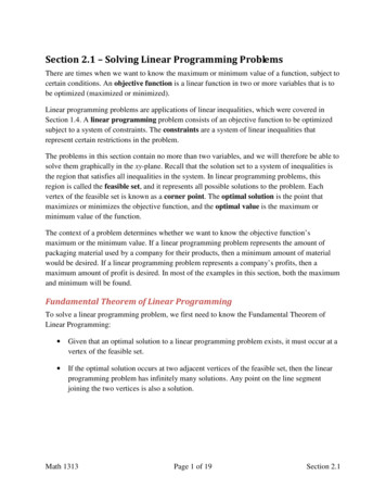
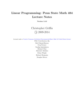
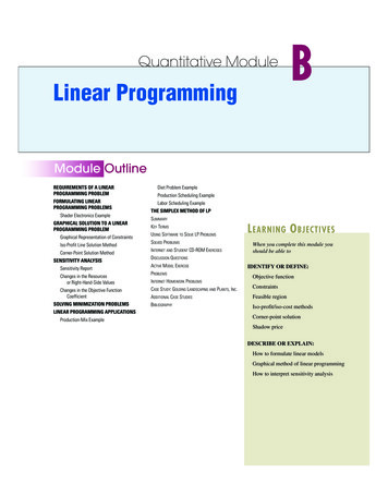
Minimizec 1 x1Subject to a11 x1a21 x1.am1 x1x1 , c 2 x2 ··· a12 x2a22 x2.am2 x2 ······ ··· x2 ,c n xna1n xna2n xn. amn xn.,xn z b1 b2. bm 0.In linear programming z, the expression being optimized, is called the objective function. The variables x1 , x2 . . . xn are called decision variables, and theirvalues are subject to m 1 constraints (every line ending with a bi , plus thenonnegativity constraint). A set of x1 , x2 . . . xn satisfying all the constraints iscalled a feasible point and the set of all such points is called the feasible region. The solution of the linear program must be a point (x1 , x2 , . . . , xn ) in thefeasible region, or else not all the constraints would be satisfied.The following example from Chapter 3 of Winston [3] illustrates that geometrically interpreting the feasible region is a useful tool for solving linearprogramming problems with two decision variables. The linear program is:Minimize4x1Subject to 3x1x1x1 x2x2 z 10 x2 53x1 , x 2 0.We plotted the system of inequalities as the shaded region in Figure 1. Sinceall of the constraints are “greater than or equal to” constraints, the shadedregion above all three lines is the feasible region. The solution to this linearprogram must lie within the shaded region.Recall that the solution is a point (x1 , x2 ) such that the value of z is thesmallest it can be, while still lying in the feasible region. Since z 4x1 x2 ,plotting the line x1 (z x2 )/4 for various values of z results in isocost lines,which have the same slope. Along these lines, the value of z is constant. InFigure 1, the dotted lines represent isocost lines for different values of z. Sinceisocost lines are parallel to each other, the thick dotted isocost line for whichz 14 is clearly the line that intersects the feasible region at the smallestpossible value for z. Therefore, z 14 is the smallest possible value of z given4
the constraints. This value occurs at the intersection of the lines x1 3 andx1 x2 5, where x1 3 and x2 2.Figure 1: The shaded region above all three solid lines is the feasible region(one of the constraints does not contribute to defining the feasible region). Thedotted lines are isocost lines. The thick isocost line that passes through theintersection of the two defining constraints represents the minimum possiblevalue of z 14 while still passing through the feasible region.1.2AssumptionsBefore we get too focused on solving linear programs, it is important to reviewsome theory. For instance, several assumptions are implicit in linear programingproblems. These assumptions are:1. Proportionality The contribution of any variable to the objective function or constraints is proportional to that variable. This implies no dis-5
counts or economies to scale. For example, the value of 8x1 is twice thevalue of 4x1 , no more or less.2. Additivity The contribution of any variable to the objective function orconstraints is independent of the values of the other variables.3. Divisibility Decision variables can be fractions. However, by using a special technique called integer programming, we can bypass this condition.Unfortunately, integer programming is beyond the scope of this paper.4. Certainty This assumption is also called the deterministic assumption.This means that all parameters (all coefficients in the objective functionand the constraints) are known with certainty. Realistically, however,coefficients and parameters are often the result of guess-work and approximation. The effect of changing these numbers can be determined withsensitivity analysis, which will be explored later in Section 9 [3].1.3Manipulating a Linear Programming ProblemMany linear problems do not initially match the canonical form presented in theintroduction, which will be important when we consider the Simplex algorithm.The constraints may be in the form of inequalities, variables may not havea nonnegativity constraint, or the problem may want to maximize z insteadof minimize z. We now consider some ways to manipulate problems into thedesired form.Constraint Inequalities We first consider the problem of making all constraints of a linear programming problem in the form of strict equalities. Byintroducing new variables to the problem that represent the difference betweenthe left and the right-hand sides of the constraints, we eliminate this concern.Subtracting a slack variable from a “greater than or equal to” constraint orby adding an excess variable to a “less than or equal to” constraint, transforms inequalities into equalities. For example, the constraint 4x1 x2 3becomes 4x1 x2 e1 3 with the addition of e1 0. If the constraint wereoriginally 4x1 x2 3, the additional surplus variable s1 must be subtracted(4x1 x2 s1 3) so that s1 can be a strictly nonnegative variable.URS Variables If a variable can be negative in the context of a linear programming problem it is called a urs (or “unrestricted in sign”) variable. By6
replacing this variable xj with x0j x00j where x0j , x00j 0, the problem fits thecanonical form.Minimization/Maximization If needed, converting a maximization problem to a minimization problem is quite simple. Given that z is an objectivefunction for a maximization problemmax z min ( z).1.4The Linear Algebra of Linear ProgrammingThe example of a canonical linear programming problem from the introductionlends itself to a linear algebra-based interpretation. As a reminder, the form ofa canonical problem is:Minimizec 1 x1Subject to a11 x1a21 x1.am1 x1x1 , c 2 x2 ··· a12 x2a22 x2.am2 x2 ······ ··· x2 ,c n xna1n xna2n xn. amn xn.,xn z b1 b2. bm 0.By applying some basic linear algebra, this problem becomes:MinimizeSubject toPnc j xjPnj 1j 1 aj xjxj z b 0 j 1, 2, . . . , n.or, more compactly,MinimizecxSubject to Axx zb 0,Here A is an mxn matrix whose j th column is aj . This matrix correspondsto the coefficients on x1 , x2 , . . . , xn in the constraints of a linear programming7
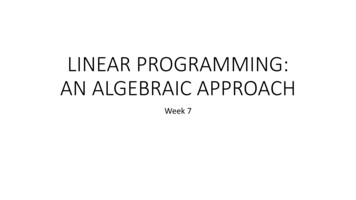
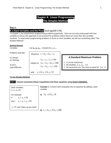
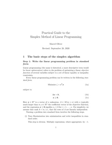
problem. The vector x is a vector of solutions to the problem, b is the righthand-side vector, and c is the cost coefficient vector. This more compact way ofthinking about linear programming problems is useful especially in sensitivityanalysis, which will be discussed in Section 9.1.5Convex Sets and DirectionsThis section defines important terms related to the feasible region of a linearprogram.Definition 1.1. A set X R is a convex set if given any two points x1and x2 in X, any convex combination of these two points is also in X. That is,λx1 (1 λ)x2 X for any λ [0, 1] [2]. See Figure 4 for an example of aconvex set.A set X is convex if the line segment connecting any two points in X is alsocontained in X. If any part of the line segment not in X, then X is said to benonconvex. Figure 2 shows an example of a nonconvex set and a convex set.The feasible region of a linear program is always a convex set. To see why thismakes sense, consider the 2-dimensional region outlined on the axes in Figure3. This region is nonconvex. In linear programming, this region could not occurbecause (from Figure 3) y mx h for c x d but y b for d x e.The constraint y mx h doesn’t hold when d x e and the constrainty b doesn’t hold when 0 x d. These sorts of conditional constraints donot occur in linear programming. A constraint cannot be valid on one regionand invalid on another.AB12Figure 2: Set 1 is an example of a nonconvex set and set 2 is an example of aconvex set. The endpoints of line segment AB are in set 1, yet the entire line isnot contained in set 1. No such line segment is possible in set 2.8
Figure 3: A nonconvex (and therefore invalid) feasible region.Definition 1.2. A point x in a convex set X is called an extreme pointof X if x cannot be represented as a strict convex combination of two distinctpoints in X [2]. A strict convex combination is a convex combination for whichλ (0, 1).Graphically, an extreme point is a corner point. We will not prove thisfact rigorously. In two dimensions, two constraints define an extreme point attheir intersection. Further, if two points x0 and x00 make up a strict convexcombination that equals x̄, then all three of these points must be defined by thesame constraints, or else they could not be colinear. However, if two constraintsdefine x̄ at their intersection, then x̄ is unique, since two lines can only intersectonce (or not at all). Since this intersection is unique, yet all three points mustlie on both constraints, x0 x00 x̄. Therefore, the strict convex combinationcan’t exist and hence corner points and extreme points are equivalent.Definition 1.3. Given a convex set, a nonzero vector d is a direction of theset if for each x0 in the set, the ray {x0 λd : λ 0} also belongs to the set.Definition 1.4. An extreme direction of a convex set is a direction of the setthat cannot be represented as a positive combination of two distinct directionsof the set.9
Figure 4: A bounded set with 4 extreme points. This set is bounded becausethere are no directions. Also, the extreme point (2, 1) is a degenerate extremepoint because it is the intersection of 3 constraints, but the feasible region isonly two-dimensional. In general, an extreme point is degenerate if the numberof intersecting constraints at that point is greater than the dimension of thefeasible region.Examples of a direction and an extreme direction can be seen in Figure 5.We need all of these definitions to state the General Representation Theorem, a building-block in linear programming. The General RepresentationTheorem states that every point in a convex set can be represented as a convex combination of extreme points, plus a nonnegative linear combination ofextreme directions. This theorem will be discussed more later.10
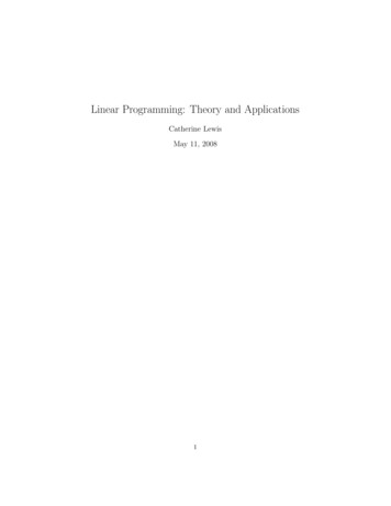
Figure 5: The shaded region in this figure is an unbounded convex set. Point Ais an example of an extreme point, vector B is an example of a direction of theset and vector C is an example of an extreme direction of the set.2Examples from Bazaraa et. al. and WinstonThe following examples deal with interpreting a word problem and setting up alinear program.2.1Examples1. Consider the problem of locating a new machine to an existing layoutconsisting of four machines. These machines are located at the following(x, y) coordinates: (3, 0), (0, 3), ( 2, 1), and (1, 4). Let the coordinatesof the new machine be (x1 , x2 ). Formulate the problem of finding anoptimal location as a linear program if the sum of the distances fromthe new machine to the existing four machines is minimized. Use streetdistance; for example, the distance from (x1 , x2 ) to the first machine at11
(3, 0) is x1 3 x2 . This means that the distance is not defined by thelength of a line between two points, rather it is the sum of the lengths ofthe horizontal and vertical components of such a line.Solution Since absolute value signs cannot be included in a linear program, recall that: x max {x, x}.With this in mind, the following linear program models the problem:MinimizeSubject tozP1 (P1 P2 ) (P3 P4 ) (P5 P6 ) (P7 P8 ) (x1 3)P1P2 x1 3 (x2 )P2 x2P3P3 (x1 1) x1 1P4P4 (x2 4) x2 4P5P5 (x1 2) x1 2P6P6 (x2 1) x2 1P7P7 (x1 ) x1P8P8 (x2 3) x2 3all variables 0.Each P2i 1 represents the horizontal distance between the new machineand the ith old machine for i 1, 2, 3, 4. Also for i 1, 2, 3, 4, P2i represents the vertical distance between the new machine and the ith oldmachine. The objective function reflects the desire to minimize total distance between the new machine and all the others. The constraints relatethe P variables to the distances in terms of x1 and x2 . Two constraintsfor each P variable allow each Pi (i 1, 2, . . . , 8) to equal the maximum12
of xj cj and (xj cj ) (for j 1, 2 and where c is the j th component of the position of one of the old machines). Since this program isa minimization problem and the smallest any of the variables can be ismax {(xj cj ), (xj cj )}, each Pi will naturally equal its least possiblevalue. This value will be the absolute value of xj cj .In the next problem we will also interpret a “real-world” situation as alinear program. Perhaps the most notable aspect of this problem is theconcept of inventory and recursion in constraints.2. A company is opening a new franchise and wants to try minimizing theirquarterly cost using linear programming. Each of their workers gets paid 500 per quarter and works 3 contiguous quarters per year. Additionally,each worker can only make 50 pairs of shoes per quarter. The demand (inpairs of shoes) is 600 for quarter 1, 300 for quarter 2, 800 for quarter 3,and 100 for quarter 4. Pairs of shoes may be put in inventory, but thiscosts 50 per quarter per pair of shoes, and inventory must be empty atthe end of quarter 4.Solution In order to minimize the cost per year, decision variables aredefined. If we letPt number of pairs of shoes during quarter t, t 1, 2, 3, 4WtIt number of workers starting work in quarter t, t 1, 2, 3, 4 number of pairs of shoes in inventory after quarter t, t 1, 2, 3, 4,the objective function is thereforemin z 50I1 50I2 50I3 1500W1 1500W2 1500W3 1500W4.Since each worker works three quarters they must be payed three timestheir quarterly rate. The objective function takes into account the salarypaid to the workers, as well as inventory costs. Next, demand for shoesmust be considered. The following constraints account for demand:13
P1I1 600 P1 600I2I3 I1 P2 300 I2 P3 800I4 I3 P4 100 0.Note these constraints are recursive, meaning they can be defined by theexpression:I n I n1 P n D nwhere Dn is just a number symbolizing demand for that quarter.Also, the workers can only make 50 pairs of shoes per quarter, which givesus the constraintsP1P2 50W1 50W3 50W4 50W2 50W4 50W1P3P4 50W3 50W1 50W2 50W4 50W3 50W2This linear program is somewhat cyclical, since workers starting work inquarter 4 can produce shoes during quarters 1 and 2. It is set up this wayin order to promote long-term minimization of cost and to emphasize thatthe number of workers starting work during each quarter should alwaysbe the optimal value, and not vary year to year.The next example is a similar type of problem. Again, decision variablemust be identified and constraints formed to meet a certain objective.However, this problem deals with a different real-world situation and it isinteresting to see the difference in the structure of the program.In the previous problem, the concepts of inventory and scheduling werekey, in the next problem, the most crucial aspect is conservation of matter.This means that several options will be provided concerning how to disposeof waste and all of the waste must be accounted for by the linear program.3. Suppose that there are m sources that generate waste and n disposal sites.The amount of waste generated at source i is ai and the capacity of site jis bj . It is desired to select appropriate transfer facilities from among Kcandidate facilities. Potential transfer facility k has fixed cost fk , capacity14
qk and unit processing cost αk per ton of waste. Let cik and c̄kj be theunit shipping costs from source i to transfer station k and from transferstation k to disposal site j respectively. The problem is to choose thetransfer facilities and the shipping pattern that minimize the total capitaland operating costs of the transfer stations plus the transportation costs.Solution As with the last problem, defining variables is the first step.wikyk tons of waste moved from i to k, 1 i m, 1 k K a binary variable that equals 1 when transfer station k is usedand 0 otherwise, 1 k Kxkj tons of waste moved from k to j, 1 k K, 1 j nThe objective function features several double sums in order to describeall the costs faced in the process of waste disposal. The objective functionis:min z XXikcik wik XXc̄kj xkj jkXkfk yk XXkαk wik .iThe first constraint equates the tons of waste coming from all the sourceswith the tons of waste going to all the disposal sites. This constraint isXwik iXxkj .jThe next constraint says that the amount of waste produced equals theamount moved to all the transfer facilities:Xwik Xai .ikNext, there must be a constraint that restricts how much waste is attransfer or disposal sites depending on their capacity. This restriction15
gives:Xxkj bj andXwik qk .ikPutting these constraints all together, the linear program is:MinimizeSubject tozPwikPiwikPkxkjPki wikP PP PPP P ik cik wik kj c̄kj xkj k fk yk ki αk wikPx kjPja i i bj qkall variables 0.Most linear program-solving software allows the user to designate certain variables as binary, so ensuring this property of yk would not be an obstacle insolving this problem.2.2DiscussionNow let’s discuss the affects altering a linear program has on the program’sfeasible region and optimal objective function value. Consider the typical linearprogram: minimize cx subject to Ax b, x 0.First, suppose that a new variable xn 1 is added to the problem. Thefeasible region gets larger or stays the same. After the addition of xn 1 thefeasible region goes up in dimension. It still contains all of its original points(where xn 1 0) but it may now also include more.The optimal objective function value of this program gets smaller or staysthe same. Since there are more options in the feasible region, there may be onethat more effectively minimizes z. If the new variable is added to z (that is,any positive value of that variable would make z larger), then that variable willequal 0 at optimality.Now, suppose that one component of the vector b, say bi , is increased byone unit to bi 1. The feasible region gets smaller or stays the same. To see thismore clearly, let y symbolize the row vector of coefficients of the constraint towhich 1 was added. The new feasible region is everything from the old feasibleregion except points that satisfy the constraint bi y · x bi 1. This is eithera positive number or zero, so therefore the feasible region gets smaller or stays16
the same.The optimal objective of this new program gets larger or stays the same. Tosatisfy the new constraint, the variables in that constraint may have to increasein value. This increase may in turn increase the value of the objective function.In general, when changes are made in the program to increase the size of thefeasible region, the optimal objective value either stays the same, or becomesmore optimal (smaller for a minimization problem, or larger for a maximizationproblem). This is because a larger feasible region presents more choices, oneof which may be better than the previous result. Conversely, when a feasibleregion decreases in size, the optimal objective value either stays the same, orbecomes less optimal.3The Theory Behind Linear Programming3.1DefinitionsNow that several examples, have been presented, it is time to explore the theorybehind linear programming more thoroughly. The climax of this chapter willbe the General Representation Theorem and to reach this end, more definitionsand theorems are necessary.Definition 3.1. A hyperplane H in Rn is a set of the form {x : px k}where p is a nonzero vector in Rn and k is a scalar.For example, {(x1 , x2 ) : (1, 0) · (x1 , x2 ) 2} is a hyperplane in R2 . Aftercompleting the dot product, it turns out that this is just the line x1 2 whichcan be plotted on the x1 x2 -plane.A hyperplane in three dimensions is a traditional plane, and in two dimensions it is a line. The purpose of this definition is to generalize the idea of aplane to more dimensions.Definition 3.2. A halfspace is a collection of points of the form {x : px k}or {x : px k}.Consider the two-dimensional halfspace {(x1 , x2 ) : (1, 0)·(x1 , x2 ) 2}. Aftercompleting the dot product, it is clear that this halfspace describes the regionwhere x1 2. On the x1 , x2 plane, this would be everything to the left of thehyperplane x1 2.A halfspace in R2 is everything on one side of a line and, similarly, in R3 ahalfspace is everything on one side of a a plane.17
Definition 3.3. A polyhedral set is the intersection of a finite number ofhalfspaces. It can be written in the form {x : Ax b} where A is an m nmatrix (where m and n are integers).Every polyhedral set is a convex set. See Figure 6 for an example of a polyhedral set. A proper face of a polyhedral set X is a set of points that corresponds tosome nonempty set of binding defining hyperplanes of X. Therefore, the highestdimension of a proper face of X is equal to dim(X)-1. An edge of a polyhedralset is a one-dimensional face of X. Extreme points are zero-dimensional facesof X, which basically summarizes the next big definition:Figure 6: This “pup tent” is an example of a polyhedral set in R3 . Point A isan extreme point because it is defined by three halfspaces: everything behindthe plane at the front of the tent, and everything below the two planes definingthe sides of the tent. The line segment from A to B is called an “edge” of thepolyhedral set. Set C is a set of points that forms a two-dimensional properface of the pup tent.Definition 3.4. Let X Rn , where n is an integer. A point x̄ X is said tobe an extreme point of set X if x̄ lies on some n linearly independent defining18
hyperplanes of X.Earlier, an extreme point was said to be a “corner point” of a feasible regionin two dimensions. The previous definition states the definition of an extremepoint more formally and generalizes it for more than two dimensions.All of the previous definitions are for the purpose of generalizing the ideaof a feasible region to more than two-dimensions. The feasible region will always be a polyhedral set, which, according to the definition, is a convex setin n dimensions. The terminology presented in these definitions is used in thestatement and proof of the General Representation Theorem, which is coveredin the next section.3.2The General Representation TheoremOne of the most important (and difficult) theorems in linear programming isthe General Representation Theorem. This theorem not only provides a way torepresent any point in a polyhedral set, but its proof also lays the groundworkfor understanding the Simplex method, a basic tool for solving linear programs.Theorem 3.1. The General Representation Theorem: Let X {x :Ax b, x 0} be a nonempty polyhedral set. Then the set of extreme pointsis not empty and is finite, say {x1 , x2 , . . . , xk }. Furthermore, the set of extremedirections is empty if and only if X is bounded. If X is not bounded, thenthe set of extreme directions is nonempty and is finite, say {d1 , d2 , . . . , dl }.Moreover, x̄ X if and only if it can be represented as a convex combination ofx1 , x2 , . . . , xk plus a nonnegative linear combination of d1 , d2 , . . . , dl , that is,x̄ kXλj x j j 1kXlXµj d jj 1λj 1,j 1λj 0,µj 0,j 1, 2, . . . , kj 1, 2, . . . , l.In sum, by visualizing an unbounded polyhedral set in two-dimensions, it isclear that any point in between extreme points can be represented as a convexcombination of those extreme points. Any other point can be represented as19
one of these convex combinations, plus a combination of multiples of extremedirections.This theorem is called “general” since it applies to either a bounded polyhedral set (in the case that µj 0 for all j) or an unbounded polyhedral set.4An Outline of the ProofThe General Representation Theorem (GRT) has four main parts. First, itstates that the number of extreme points in X is nonempty and finite. Next, ifX is bounded then the set of extreme directions of X is empty. Further, if X isnot bounded, then the set of extreme directions is nonempty and finite. Finally,the GRT states that x̄ X if and only if it can be represented as a convexcombination of extreme points of X and a nonnegative linear combination ofextreme directions of X. We will explore the proofs of these parts in sequence.Since the last part of the GRT is a “if and only if” theorem, it must beproven both ways. Proving that if a point x can be represented as a convexcombination of extreme points of a set X, plus a combination of multiples ofextreme directions of X, then x X (the “backward” proof), is simple. Beforewe do that, however, we must prove the first two parts of the GRT: First, we want to prove that there are a finite number of extreme points inthe set X. We do this by moving along extreme directions until reaching apoint that has n linearly independent defining hyperplanes, where n is just an integer. Thus there is at least 1 extreme point. Furthermore, m nisnfinite, so the number of extreme points is finite. Prove that there are a finite number of extreme directions in the set X.The argument here is similar to proving that there are a finite number ofextreme points.Next
Minimize c1x1 c2x2 cnxn z Subject to a11x1 a12x2 a1nxn b1 a21x1 a22x2 a2nxn b2 am1x1 am2x2 amnxn bm x1; x2; :::; xn 0: In linear programming z, the expression being optimized, is called the objec-tive function. The variables x1;x2:::xn are called decision variables, and their values are