Transcription
Kreith, F.; Boehm, R.F.; et. al. “Heat and Mass Transfer”Mechanical Engineering HandbookEd. Frank KreithBoca Raton: CRC Press LLC, 1999c1999 by CRC Press LLC
Heat and Mass TransferFrank KreithUniversity of ColoradoRobert F. BoehmUniversity of Nevada-Las Vegas4.1Introduction Fourier’s Law Insulations The Plane Wall atSteady State Long, Cylindrical Systems at Steady State TheOverall Heat Transfer Coefficient Critical Thickness ofInsulation Internal Heat Generation Fins Transient Systems Finite-Difference Analysis of ConductionGeorge D. RaithbyUniversity of WaterlooK. G. T. HollandsUniversity of WaterlooN. V. Suryanarayana4.24.3Van P. CareyJohn C. Chen4.44.5Heat Exchangers .4-1184.6Temperature and Heat Transfer Measurements.4-182Compact Heat Exchangers Shell-and-Tube Heat ExchangersUniversity of PennsylvaniaRam K. ShahTemperature Measurement Heat Flux Sensor EnvironmentalErrors Evaluating the Heat Transfer CoefficientDelphi Harrison Thermal SystemsKenneth J. Bell4.7Oklahoma State UniversityStanford UniversityUniversity of California at Los Angeles4.8Larry W. SwansonHeat Transfer Research InstituteVincent W. AntonettiPoughkeepsie, New YorkApplications.4-240Enhancement Cooling Towers Heat Pipes CoolingElectronic EquipmentArthur E. BerglesRensselaer Polytechnic InstituteMass Transfer .4-206Introduction Concentrations, Velocities, and Fluxes Mechanisms of Diffusion Species Conservation Equation Diffusion in a Stationary Medium Diffusion in a MovingMedium Mass ConvectionRobert J. MoffatAnthony F. MillsPhase-Change .4-82Boiling and Condensation Particle Gas Convection Meltingand FreezingLehigh UniversityNoam LiorRadiation .4-56Nature of Thermal Radiation Blackbody Radiation Radiative Exchange between Opaque Surfaces RadiativeExchange within Participating MediaPennsylvania State UniversityUniversity of California at BerkeleyConvection Heat Transfer .4-14Natural Convection Forced Convection — External Flows Forced Convection — Internal FlowsMichigan Technological UniversityMichael F. ModestConduction Heat Transfer.4-24.9Non-Newtonian Fluids — Heat Transfer .4-279Introduction Laminar Duct Heat Transfer — Purely Viscous,Time-Independent Non-Newtonian Fluids Turbulent DuctFlow for Purely Viscous Time-Independent Non-NewtonianFluids Viscoelastic Fluids Free Convection Flows and HeatTransferThomas F. Irvine, Jr.State University of New York, Stony BrookMassimo CapobianchiState University of New York, Stony Brook 1999 by CRC Press LLC4-1
4-2Section 44.1 Conduction Heat TransferRobert F. BoehmIntroductionConduction heat transfer phenomena are found throughout virtually all of the physical world and theindustrial domain. The analytical description of this heat transfer mode is one of the best understood.Some of the bases of understanding of conduction date back to early history. It was recognized that byinvoking certain relatively minor simplifications, mathematical solutions resulted directly. Some of thesewere very easily formulated. What transpired over the years was a very vigorous development ofapplications to a broad range of processes. Perhaps no single work better summarizes the wealth of thesestudies than does the book by Carslaw and Jaeger (1959). They gave solutions to a broad range ofproblems, from topics related to the cooling of the Earth to the current-carrying capacities of wires. Thegeneral analyses given there have been applied to a range of modern-day problems, from laser heatingto temperature-control systems.Today conduction heat transfer is still an active area of research and application. A great deal ofinterest has developed in recent years in topics like contact resistance, where a temperature differencedevelops between two solids that do not have perfect contact with each other. Additional issues of currentinterest include non-Fourier conduction, where the processes occur so fast that the equation describedbelow does not apply. Also, the problems related to transport in miniaturized systems are garnering agreat deal of interest. Increased interest has also been directed to ways of handling composite materials,where the ability to conduct heat is very directional.Much of the work in conduction analysis is now accomplished by use of sophisticated computercodes. These tools have given the heat transfer analyst the capability of solving problems in nonhomogenous media, with very complicated geometries, and with very involved boundary conditions. It is stillimportant to understand analytical ways of determining the performance of conducting systems. At theminimum these can be used as calibrations for numerical codes.Fourier’s LawThe basis of conduction heat transfer is Fourier’s Law. This law involves the idea that the heat flux isproportional to the temperature gradient in any direction n. Thermal conductivity, k, a property ofmaterials that is temperature dependent, is the constant of proportionality.qk - kA¶T¶n(4.1.1)In many systems the area A is a function of the distance in the direction n. One important extension isthat this can be combined with the first law of thermodynamics to yield the heat conduction equation.For constant thermal conductivity, this is given asÑ2T q G 1 ¶T a ¶tk(4.1.2)In this equation, a is the thermal diffusivity and q̇G is the internal heat generation per unit volume.Some problems, typically steady-state, one-dimensional formulations where only the heat flux is desired,can be solved simply from Equation (4.1.1). Most conduction analyses are performed with Equation(4.1.2). In the latter, a more general approach, the temperature distribution is found from this equationand appropriate boundary conditions. Then the heat flux, if desired, is found at any location usingEquation (4.1.1). Normally, it is the temperature distribution that is of most importance. For example, 1999 by CRC Press LLC
4-3Heat and Mass Transferit may be desirable to know through analysis if a material will reach some critical temperature, like itsmelting point. Less frequently the heat flux is desired.While there are times when it is simply desired to understand what the temperature response of astructure is, the engineer is often faced with a need to increase or decrease heat transfer to some specificlevel. Examination of the thermal conductivity of materials gives some insight into the range of possibilities that exist through simple conduction.Of the more common engineering materials, pure copper exhibits one of the higher abilities to conductheat with a thermal conductivity approaching 400 W/m2 K. Aluminum, also considered to be a goodconductor, has a thermal conductivity a little over half that of copper. To increase the heat transfer abovevalues possible through simple conduction, more-involved designs are necessary that incorporate a varietyof other heat transfer modes like convection and phase change.Decreasing the heat transfer is accomplished with the use of insulations. A separate discussion ofthese follows.InsulationsInsulations are used to decrease heat flow and to decrease surface temperatures. These materials arefound in a variety of forms, typically loose fill, batt, and rigid. Even a gas, like air, can be a goodinsulator if it can be kept from moving when it is heated or cooled. A vacuum is an excellent insulator.Usually, though, the engineering approach to insulation is the addition of a low-conducting material tothe surface. While there are many chemical forms, costs, and maximum operating temperatures ofcommon forms of insulations, it seems that when a higher operating temperature is required, many timesthe thermal conductivity and cost of the insulation will also be higher.Loose-fill insulations include such materials as milled alumina-silica (maximum operating temperatureof 1260 C and thermal conductivities in the range of 0.1 to 0.2 W/m2 K) and perlite (maximum operatingtemperature of 980 C and thermal conductivities in the range of 0.05 to 1.5 W/m2 K). Batt-typeinsulations include one of the more common types — glass fiber. This type of insulation comes in avariety of densities, which, in turn, have a profound affect on the thermal conductivity. Thermal conductivities for glass fiber insulations can range from about 0.03 to 0.06 W/m2K. Rigid insulations showa very wide range of forms and performance characteristics. For example, a rigid insulation in foamform, polyurethane, is very lightweight, shows a very low thermal conductivity (about 0.02 W/m2 K),but has a maximum operating temperature only up to about 120 C. Rigid insulations in refractory formshow quite different characteristics. For example, high-alumina brick is quite dense, has a thermalconductivity of about 2 W/m2 K, but can remain operational to temperatures around 1760 C. Manyinsulations are characterized in the book edited by Guyer (1989).Often, commercial insulation systems designed for high-temperature operation use a layered approach.Temperature tolerance may be critical. Perhaps a refractory is applied in the highest temperature region,an intermediate-temperature foam insulation is used in the middle section, and a high-performance, lowtemperature insulation is used on the outer side near ambient conditions.Analyses can be performed including the effects of temperature variations of thermal conductivity.However, the most frequent approach is to assume that the thermal conductivity is constant at sometemperature between the two extremes experienced by the insulation.The Plane Wall at Steady StateConsider steady-state heat transfer in a plane wall of thickness L, but of very large extent in both otherdirections. The wall has temperature T1 on one side and T2 on the other. If the thermal conductivity isconsidered to be constant, then Equation (4.1.1) can be integrated directly to give the following result:qk kA(T - T2 )L 1This can be used to determine the steady-state heat transfer through slabs. 1999 by CRC Press LLC(4.1.3)
4-4Section 4An electrical circuit analog is widely used in conduction analyses. This is realized by considering thetemperature difference to be analogous to a voltage difference, the heat flux to be like current flow, andthe remainder of Equation (4.1.3) to be like a thermal resistance. The latter is seen to beRk LkA(4.1.4)Heat transfer through walls made of layers of different types of materials can be easily found by summingthe resistances in series or parallel form, as appropriate.In the design of systems, seldom is a surface temperature specified or known. More often, the surfaceis in contact with a bulk fluid, whose temperature is known at some distance from the surface. Convectionfrom the surface is then represented by Newton’s law of cooling:q hc A(Ts - T )(4.1.5)This equation can also be represented as a temperature difference divided by a thermal resistance, whichis 1/ hcA . It can be shown that a very low surface resistance, as might be represented by phase changephenomena, has the effect of imposing the fluid temperature directly on the surface. Hence, usually aknown surface temperature results from a fluid temperature being imposed directly on the surface througha very high heat transfer coefficient. For this reason, in the later results given here, particularly thosefor transient systems, a convective boundary will be assumed. For steady results this is less importantbecause of the ability to add resistances through the circuit analogy.Long, Cylindrical Systems at Steady StateFor long (L) annular systems at steady-state conditions with constant thermal conductivities, the followingtwo equations are the appropriate counterparts to Equations (4.1.3) and (4.1.4). The heat transfer can beexpressed asqk 2 pLk(T - T2 )ln r2 r1 1[](4.1.6)Here, r1 and r2 represent the radii of annular section. A thermal resistance for this case is as shown below.Rk [ln r2 r12pLk](4.1.7)The Overall Heat Transfer CoefficientThe overall heat transfer coefficient concept is valuable in several aspects of heat transfer. It involvesa modified form of Newton’s law of cooling, as noted above, and it is written asQ U ADT(4.1.8)In this formulation U is the overall heat transfer coefficient based upon the area A. Because the areafor heat transfer in a problem can vary (as with a cylindrical geometry), it is important to note that theU is dependent upon which area is selected. The overall heat transfer coefficient is usually found froma combination of thermal resistances. Hence, for a common series-combination-circuit analog, the U Aproduct is taken as the sum of resistances. 1999 by CRC Press LLC
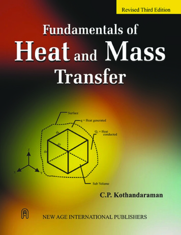
4-5Heat and Mass TransferUA 1 nåR1Rtotal(4.1.9)ii 1To show an example of the use of this concept, consider Figure 4.1.1.FIGURE 4.1.1. An insulated tube with convective environments on both sides.For steady-state conditions, the product U A remains constant for a given heat transfer and overalltemperature difference. This can be written asU1 A1 U2 A2 U3 A3 U A(4.1.10)If the inside area, A1, is chosen as the basis, the overall heat transfer coefficient can then be expressed asU1 1r1 ln(r2 r1 ) r1 ln(r3 r2 )r1 1hc,ikpipekinsr3 hc,o(4.1.11)Critical Thickness of InsulationSometimes insulation can cause an increase in heat transfer. This circumstance should be noted in orderto apply it when desired and to design around it when an insulating effect is needed. Consider thecircumstance shown in Figure 4.1.1. Assume that the temperature is known on the outside of the tube(inside of the insulation). This could be known if the inner heat transfer coefficient is very large and thethermal conductivity of the tube is large. In this case, the inner fluid temperature will be almost the sameas the temperature of the inner surface of the insulation. Alternatively, this could be applied to a coating(say an electrical insulation) on the outside of a wire. By forming the expression for the heat transferin terms of the variables shown in Equation (4.1.11), and examining the change of heat transfer withvariations in r3 (that is, the thickness of insulation) a maximum heat flow can be found. While simpleresults are given many texts (showing the critical radius as the ratio of the insulation thermal conductivityto the heat transfer coefficient on the outside), Sparrow (1970) has considered a heat transfer coefficientthat varies as hc,o r3- m T3 – Tf,o n. For this case, it is found that the heat transfer is maximized at 1999 by CRC Press LLC
4-6Section 4r3 rcrit [(1 - m) (1 n)]kinshc,o(4.1.12)By examining the order of magnitudes of m, n, kins, and hc,o the critical radius is found to be oftenon the order of a few millimeters. Hence, additional insulation on small-diameter cylinders such as smallgauge electrical wires could actually increase the heat dissipation. On the other hand, the addition ofinsulation to large-diameter pipes and ducts will almost always decrease the heat transfer rate.Internal Heat GenerationThe analysis of temperature distributions and the resulting heat transfer in the presence of volume heatsources is required in some circumstances. These include phenomena such as nuclear fission processes,joule heating, and microwave deposition. Consider first a slab of material 2L thick but otherwise verylarge, with internal generation. The outside of the slab is kept at temperature T1. To find the temperaturedistribution within the slab, the thermal conductivity is assumed to be constant. Equation (4.1.2) reducesto the following:d 2 T q G 0dx 2k(4.1.13)Solving this equation by separating variables, integrating twice, and applying boundary conditions givesT ( x ) - T1 q G L2 é æ x ö 2 ùê1 ú2k ë è L ø û(4.1.14)A similar type of analysis for a long, cylindrical element of radius r1 gives2q G r12 é æ r ö ùê1 úT (r ) - T1 4k ê çè r1 ø úëû(4.1.15)Two additional cases will be given. Both involve the situation when the heat generation rate isdependent upon the local temperature in a linear way (defined by a slope b), according to the followingrelationship:[]q G q G,o 1 b(T - To )(4.1.16)For a plane wall of 2L thickness and a temperature of T1 specified on each surfaceT ( x ) - To 1 b cos mx T1 - To 1 bcos mL(4.1.17)For a similar situation in a long cylinder with a temperature of T1 specified on the outside radius r1T (r ) - To 1 b J o (mr ) T1 - To 1 bJ o (mr1 ) 1999 by CRC Press LLC(4.1.18)
4-7Heat and Mass TransferIn Equation (4.1.18), the Jo is the typical notation for the Bessel function. Variations of this function aretabulated in Abramowitz and Stegun (1964). In both cases the following holds:mºbq G,okFinsFins are widely used to enhance the heat transfer (usually convective, but it could also be radiative)from a surface. This is particularly true when the surface is in contact with a gas. Fins are used on aircooled engines, electronic cooling forms, as well as for a number of other applications. Since the heattransfer coefficient tends to be low in gas convection, area is added in the form of fins to the surface todecrease the convective thermal resistance.The simplest fins to analyze, and which are usually found in practice, can be assumed to be onedimensional and constant in cross section. In simple terms, to be one-dimensional, the fins have to belong compared with a transverse dimension. Three cases are normally considered for analysis, and theseare shown in Figure 4.1.2. They are the insulated tip, the infinitely long fin, and the convecting tip fin.FIGURE 4.1.2. Three typical cases for one-dimensional, constant-cross-section fins are shown.For Case, I, the solution to the governing equation and the application of the boundary conditions ofthe known temperature at the base and the insulated tip yieldsq qb Case I:cosh m( L - x )cosh mL(4.1.19)For the infinitely long case, the following simple form results:q( x ) q b e - mxCase II:(4.1.20)The final case yields the following result:Case III:q( x ) q bmL cosh m( L - x ) Bi sinh m( L - x )mL cosh mL Bi sinh mLwhereBi º hc L k 1999 by CRC Press LLC(4.1.21)
4-8Section 4In all three of the cases given, the following definitions apply:q º T ( x ) - T ,q b º T ( x 0) - T ,andm2 ºhc PkAHere A is the cross section of the fin parallel to the wall; P is the perimeter around that area.To find the heat removed in any of these cases, the temperature distribution is used in Fourier’s law,Equation (4.1.1). For most fins that truly fit the one-dimensional assumption (i.e., long compared withtheir transverse dimensions), all three equations will yield results that do not differ widely.Two performance indicators are found in the fin literature. The fin efficiency is defined as the ratioof the actual heat transfer to the heat transfer from an ideal fin.hºqactualqideal(4.1.22)The ideal heat transfer is found from convective gain or loss from an area the same size as the fin surfacearea, all at a temperature Tb. Fin efficiency is normally used to tabulate heat transfer results for varioustypes of fins, including ones with nonconstant area or which do not meet the one-dimensional assumption.An example of the former can be developed from a result given by Arpaci (1966). Consider a straightfin of triangular profile, as shown in Figure 4.1.3. The solution is found in terms of modified Besselfunctions of the first kind. Tabulations are given in Abramowitz and Stegun (1964).h ( L1 2I1 2 m() L1 2 Io 2 m L1 2m)(4.1.23) º 2hc L kb .Here, mThe fin effectiveness, e, is defined as the heat transfer from the fin compared with the bare-surfacetransfer through the same base area.FIGURE 4.1.3. Two examples of fins with a cross-sectional area that varies with distance from the base. (a) Straighttriangular fin. (b) Annular fin of constant thickness. 1999 by CRC Press LLC
4-9Heat and Mass Transfere qfqactual qbare base hc A(Tb - T )(4.1.24)Carslaw and Jaeger (1959) give an expression for the effectiveness of a fin of constant thickness arounda tube (see Figure 4.1.3) This is given as (m º 2hc kb ).e 2 I1 (m r2 ) K1 (m r1 ) - K1 (m r2 ) I1 (m r1 )m b Io (m r1 ) K1 (m r2 ) K o (m r1 ) I1 (m r2 )(4.1.25)Here the notations I and K denote Bessel functions that are given in Abramowitz and Stegun (1964).Fin effectiveness can be used as one indication whether or not fins should be added. A rule of thumbindicates that if the effectiveness is less than about three, fins should not be added to the surface.Transient SystemsNegligible Internal ResistanceConsider the transient cooling or heating of a body with surface area A and volume V. This is takingplace by convection through a heat transfer coefficient hc to an ambient temperature of T . Assume thethermal resistance to conduction inside the body is significantly less than the thermal resistance toconvection (as represented by Newton’s law of cooling) on the surface of the body. This ratio is denotedby the Biot number, Bi.Bi Rk hc (V A) Rck(4.1.26)The temperature (which will be uniform throughout the body at any time for this situation) responsewith time for this system is given by the following relationship. Note that the shape of the body is notimportant — only the ratio of its volume to its area matters.T (t ) - T e - hc At rVcTo - T (4.1.27)Typically, this will hold for the Biot number being less than (about) 0.1.Bodies with Significant Internal ResistanceWhen a body is being heated or cooled transiently in a convective environment, but the internal thermalresistance of the body cannot be neglected, the analysis becomes more complicated. Only simplegeometries (a symmetrical plane wall, a long cylinder, a composite of geometric intersections of thesegeometries, or a sphere) with an imposed step change in ambient temperature are addressed here.The first geometry considered is a large slab of minor dimension 2L. If the temperature is initiallyuniform at To, and at time 0 it begins convecting through a heat transfer coefficient to a fluid at T , thetemperature response is given by q 2æösin l n Lå çè l L sin l L cos l L ø exp(-l L Fo) cos(l x)n 1nn2 2nn(4.1.28)nand the ln are the roots of the transcendental equation: lnL tan lnL Bi. The following definitions hold: 1999 by CRC Press LLC
4-10Section 4Bi ºhc LkFo ºatL2qºT - T To - T The second geometry considered is a very long cylinder of diameter 2R. The temperature responsefor this situation is q 2Bi(å (l Rn 1)exp - l2n R 2 Fo J o (l n r )2n2(4.1.29)) Bi J o (l n R)2Now the ln are the roots of lnR J1(lnR) Bi Jo (lnR) 0, andBi hc RkFo atR2q T - T To - T The common definition of Bessel’s functions applies here.For the similar situation involving a solid sphere, the following holds: q 2sin(l n R) - l n R cos(l n R)å l R - sin(l R) cos(l R) exp(-l R Fo)n 1nn2nn2sin(l n r )l nr(4.1.30)and the ln are found as the roots of lnR cos lnR (1 – Bi) sin lnR. Otherwise, the same definitions aswere given for the cylinder hold.Solids that can be envisioned as the geometric intersection of the simple shapes described above canbe analyzed with a simple product of the individual-shape solutions. For these cases, the solution isfound as the product of the dimensionless temperature functions for each of the simple shapes withappropriate distance variables taken in each solution. This is illustrated as the right-hand diagram inFigure 4.1.4. For example, a very long rod of rectangular cross section can be seen as the intersectionof two large plates. A short cylinder represents the intersection of an infinitely long cylinder and a plate.The temperature at any location within the short cylinder isq 2 R,2 L Rod q Infinite 2 R Rod q 2 L Plate(4.1.31)Details of the formulation and solution of the partial differential equations in heat conduction arefound in the text by Arpaci (1966).Finite-Difference Analysis of ConductionToday, numerical solution of conduction problems is the most-used analysis approach. Two generaltechniques are applied for this: those based upon finite-difference ideas and those based upon finiteelement concepts. General numerical formulations are introduced in other sections of this book. In thissection, a special, physical formulation of the finite-difference equations to conduction phenomena isbriefly outlined.Attention is drawn to a one-dimensional slab (very large in two directions compared with thethickness). The slab is divided across the thickness into smaller subslabs, and this is shown in Figure4.1.5. All subslabs are thickness Dx except for the two boundaries where the thickness is Dx/2. Acharacteristic temperature for each slab is assumed to be represented by the temperature at the slabcenter. Of course, this assumption becomes more accurate as the size of the slab becomes smaller. With 1999 by CRC Press LLC
4-11Heat and Mass TransferFIGURE 4.1.4. Three types of bodies that can be analyzed with results given in this section. (a) Large plane wallof 2L thickness; (b) long cylinder with 2R diameter; (c) composite intersection.FIGURE 4.1.5. A one-dimensional finite differencing of a slab with a general interior node and one surface nodedetailed.the two boundary-node centers located exactly on the boundary, a total of n nodes are used (n – 2 fullnodes and one half node on each of the two boundaries).In the analysis, a general interior node i (this applies to all nodes 2 through n – 1) is considered foran overall energy balance. Conduction from node i – 1 and from node i 1 as well as any heat generationpresent is assumed to be energy per unit time flowing into the node. This is then equated to the timerate of change of energy within the node. A backward difference on the time derivative is applied here,and the notation Ti ; Ti (t Dt) is used. The balance gives the following on a per-unit-area basis:Ti - 1 - Ti Ti 1 - Ti T - Ti q G,i Dx rDxc p iDx kDx k Dt(4.1.32)In this equation different thermal conductivities have been used to allow for possible variations inproperties throughout the solid.The analysis of the boundary nodes will depend upon the nature of the conditions there. For thepurposes of illustration, convection will be assumed to be occurring off of the boundary at node 1. Abalance similar to Equation (4.1.32) but now for node 1 gives the following: 1999 by CRC Press LLC
4-12Section 4T - T1 T2 - T1 DxDx T - T q G,1 r cp 1 11 hcDx k 22Dt(4.1.33)After all n equations are written, it can be seen that there are n unknowns represented in theseequations: the temperature at all nodes. If one or both of the boundary conditions are in terms of aspecified temperature, this will decrease the number of equations and unknowns by one or two, respectively. To determine the temperature as a function of time, the time step is arbitrarily set, and all thetemperatures are found by simultaneous solution at t 0 Dt. The time is then advanced by Dt and thetemperatures are then found again by simultaneous solution.The finite difference approach just outlined using the backward difference for the time derivative istermed the implicit technique, and it results in an n n system of linear simultaneous equations. If theforward difference is used for the time derivative, then only one unknown will exist in each equation.This gives rise to what is called an explicit or “marching” solution. While this type of system is morestraightforward to solve because it deals with only one equation at a time with one unknown, a stabilitycriterion must be considered which limits the time step relative to the distance step.Two- and three-dimensional problems are handled in conceptually the same manner. One-dimensionalheat fluxes between adjoining nodes are again considered. Now there are contributions from each of thedimensions represented. Details are outlined in the book by Jaluria and Torrance (1986).Defining TermsBiot number: Ratio of the internal (conductive) resistance to the external (convective) resistance froma solid exchanging heat with a fluid.Fin: Additions of material to a surface to increase area and thus decrease the external thermal resistancefrom convecting and/or radiating solids.Fin effectiveness: Ratio of the actual heat transfer from a fin to the heat transfer from the same crosssectional area of the wall without the fin.Fin efficiency: Ratio of the actual heat transfer from a fin to the heat transfer from a fin with the samegeometry but completely at the base temperature.Fourier’s law: The fundamental law of heat conduction. Relates the local temperature gradient to thelocal heat flux, both in the same direction.Heat conduction equation: A partial differential equation in temperature, spatial variables, time, andproperties that, when solved with appropriate boundary and initial conditions, describes thevariation of temperature in a conducting medium.Overall heat transfer coefficient: The analogous quantity to the heat transfer coefficient found inconvection (Newton’s law of cooling) that represents the overall combination of several thermalresistances, both conductive and convective.Thermal conductivity: The property of a material that relates a temperature gradient to a heat flux.Dependent upon temperature.ReferencesAbramowitz, M. and Stegun, I. 1964. Handbook of Mathematical Functions with Formulas, Graphs,and Mathematical Tables. National Bureau of Standards, Applied Mathematics Series 55.Arpaci, V. 1966. Conduction Heat Transfer, Addison-Wesley, Reading, MA.Carslaw, H.S. and Jaeger, J.C. 1959. Conduction of Heat in Solids, 2nd ed., Oxford University Press,London.
4.1Conduction Heat Transfer Robert F. Boehm Introduction Conduction heat transfer phenomena are found throughout virtually all of the physical world and the industrial domain. The analytical description of this heat transfer mode is one of the best understood. Some of the bases o