Transcription
10-110. CONSOLIDATION10.1INFLUENCE OF DRAINAGE ON RATE OF SETTLEMENTWhen a saturated stratum of sandy soil is subjected to a stress increase, such as thatcaused by the erection of a building on the ground surface, the pore water pressure is increased.This increase in pore pressure leads to drainage of some water from the voids of the soil. Becauseof the relatively high permeability of the sandy soil this drainage process will occur quite quickly.In other words the pore pressure increase will dissipate rapidly. As a consequence of the drainageof some water from the soil, volume change will occur and settlement will take place.When a saturated stratum of clayey soil is subjected to a stress increase, the dissipationof the excess pore pressure generated will take place much more slowly because of the relativelylow permeability of the clayey soil. This means that the settlement, caused by the drainage ofsome water from the voids of the soil, will take place gradually over a long period of time.Fig. 10.1(a) represents a rigid but smooth walled container which is filled with saturatedsoil. The container is sealed by means of a membrane covering the upper surface of the soil. Auniform pressure of σ is applied to the top of the soil. Since the soil is saturated and thecontainer is rigid no settlement of the soil will be observed. If the pore pressure change within thesoil was observed it would be found to equal the applied stress σ. Since the applied (total) stressand the pore pressure both increase by equal amounts, there will be no change in effective stress.The absence of any observed settlement is therefore consistent with the principle of effectivestress, which requires that volume change will occur only as a result of an effective stress change.In Fig. 10.1(b) an opening has been provided in the membrane to enable water to beexpelled or drained from the container of soil. Under the effect of the increase in pore pressure u ( σ), water will be expelled from the soil and this drainage of water will continue until thewater pressure decreases to the equilibrium value prevailing before the stress change of σ wasapplied to the soil. This means that the pore pressure change finally will be zero. Since the totalstress has increased by σ the effective stress will also increase by σ. In response to thiseffective stress change, settlement of the soil will occur, the amount depending upon thecompressibility of the soil.These observations illustrate that in a one dimensional compression situation for asaturated soil, settlement of the soil in response to an applied stress occurs only when water isallowed to be expelled from the soil.
10-2(a) Sample sealed, drainage prevented(b) drainage permittedFig.10.1 Influence of Drainage upon stress changesFig 10.2 Vertical stress changes during consolidationThe stress changes throughout the depth of a soil layer in a one dimensional field situation areillustrated in Fig. 10.2. The initial conditions ar represented in Fig. 10.2(a). Since the water table
10-3is coincident with the ground surface the initial pore pressure ui at any depth z below the groundsurface isui ρw g zthe initial total vertical stress σi isσi ρ sat g zand the initial effective vertical stress σ'i isσ'i σi - ui ρ sat g z - ρw g zρb g zwhere ρb is the buoyant density of the soil. The distribution of this effective stress throughout thedepth of soil is shown by the hatched area.In Fig. 10.2(b) a stress of σ has been applied over the ground surface. The stressdiagram has been drawn for the instant following the application of load before any water hasbeen expelled from the soil. The pore pressure will increase by an amount equal to the appliedstress as in the case of Fig. 10.1(a). The pore pressure u at any depth z below the ground surfaceisu ui uρw g z σand the effective stress is the same as that before the load application.Under the effect of the additional (excess hydrostatic) pore pressure, water will beexpelled from the soil. Water will be expelled through the upper boundary of the soil and, if theunderlying rock is pervious, through the lower boundary as well. This drainage of water willcontinue until the pore pressure distribution coincides with that which existed before the surfacestress was applied as shown in Fig. 10.2(c). This means that the stress σ which was originallycarried as a pore pressure u has now been transferred to effective stress. The final effectivestress σ'f at any depth z isσ'f σ'i σρb g z σ
10-4As a result of the increase σ in effective stress the soil will undergo a volume decreaseas a consequence of the expulsion of water from the soil and a time dependent settlement of theground surface would be observed. The process of gradual transfer of stress from the porepressure to effective stress with the associated volume change is referred to as consolidation. Therate at which the settlement occurs depends upon the rate at which water is expelled from the soiland this depends upon the total head gradient and the permeability of the soil.6.2USE OF A RHEOLOGICAL MODELAn understanding of the time dependent nature of the settlement for a consolidating soilmay be assisted by considering the consolidation process a rheological model. A simple modelthat is often used is the Kelvin model (Fig. 10.3) which consists of a linear spring and a dashpot inparallel. The spring constant (E) and the dashpot constant (η) are defined as followswhere-σs EσD η (dε/dt)σs stress in the springσD stress in the dashpotε straint timeε(10.1)(10.2)If a stress ( σ) is applied to the model and remains constant σ σs σD E ε η (dε/dt)(10.3)-Assuming that the strain is zero at time zero, the solution to this equation isε --( σ/E) (1 - e - (E/η)t)which demonstrates the time dependency of the strain.(10.4)
10-5Fig. 10.3 Kelvin ModelFig. 10.4In the analogy provided by use of the Kelvin model the stress in the spring (σs) can be interpretedas effective stress in the soil and the stress in the dashpot (σD) may be interpreted as the porewater pressure.
10-6EXAMPLEIn a Kelvin model evaluate the stresses in the spring and in the dashpot (as proportions ofthe applied stress) as a function of time. The spring constant (E) is 1 MPa and the dashpotconstant (η) is 1011 Ns/m2.From equations (10.4) and (10.1)σs-- E e σ (1 - e - (E/η)t) σ - σs σ e - (E/η)t)and from equation (10.3)σD-Expressing σs and σD as proportions of σ-σs/ σ 1 - e- (E/η)t)σD/ σ e - (E/η)t) -(10.5)(10.6)1 - (σs/ σ)The time variations in σs and σD may be found from equations (10.5) and (10.6)-following substitution for the given values of E and η. The single curve representing variations inboth stresses has been plotted in Fig. 10.4.10.3CONSOLIDATION AS A SEEPAGE PROBLEMThe seepage of water from the soil during consolidation may be represented by means ofa head diagram of the type shown in Fig. 5.5. The problem will be illustrated for the situationshown in Fig. 10.5., in which a compressible clay is sandwiched between two relativelyincompressible sand layers, the water table being at the ground surface.Before the application of the surface pressure a hydrostatic pore pressure distributionprevails throughout the water in the voids of the soils. In other words the pressure head line isrepresented by line ACFB. The elevation head line from the arbitrarily chosen datum is given byline GH. The total head line is therefore HIKB. Since the total head has a constant value (equalto GB) throughout the depth of soil considered, no seepage will take place.
10-7As discussed in Section 10.1 immediately following the application of a wide surfacepressure σ to the ground surface the pore pressure in the saturated clay will rise by an amount u where u σIn other words the pressure head in the clay will increase by an amount ( u/ρw g).Because of the relatively high permeability of the sand the pore pressure increase will dissipatevery rapidly in the sand. The pressure in the sand will be transferred to effective stress almostimmediately. For this reason no pressure head increase has been drawn for the pore water in thesand. The new pressure head diagram is now represented by ACDEFB.If the elevation head is added to the pressure head the total head line HIJLKB isobtained. This line shows that there are sudden changes in total head at the upper and lowerboundaries of the clay layer. Because of the very large total head gradients (theoretically infinity)at these locations water will be expelled from the clay into the sand layers. This expulsion ofwater commences at the two boundaries of the clay layer and works progressively in towards thecentre of the clay. As the water is expelled the excess hydrostatic pore pressure decreases, thetotal head decreases, the total head gradient decreases and consequently the rate at which thewater is expelled decreases. This unsteady seepage situation is represented by the total head linesfor various times which are drawn for the upper portion of the clay in the IJLK portion of thediagram in Fig. 10.5. The total head line gradually approaches line IK as time elapses and finallycoincides with it as the total head gradient becomes zero and the expulsion of water ceases. Atthis stage the original excess hydrostatic pore pressure ( u) has been fully transferred to effectivestress.The rate at which this process of consolidation proceeds depends upon a number offactors such as the soil properties, the layer thickness and the boundary conditions. These areexamined qualitatively in Section 10.4 and quantitatively in Section 10.5.10.4FACTORS AFFECTING THE RATE OF CONSOLIDATION10.4.1PermeabilityAn increase in permeability of the consolidating soil would lead to an increase in the rateof seepage flow, other factors remaining constant. With the greater rate of expulsion of
10-8Fig. 10.5 Head Diagram for ConsolidationFig. 10.6 Element of Soil in a Consolidating Layer
10-9water from the soil the pore pressures will dissipate more rapidly. This means that a more rapidrate of consolidation occurs.10.4.2CompressibilityA greater compressibility leads to a greater decrease in the void space of the soil for aparticular stress change. This means that a greater volume of water must be expelled from the soiland this will require a longer time. Consequently a lower rate of consolidation will result.10.4.3Layer ThicknessAn increase in the layer thickness leads to a decrease in the total head gradient during thestage of pore water expulsion. It also means an increase in the volume of water to be expelled andboth of these effects lead to a lower rate of consolidation.10.4.4Boundary ConditionsThe presence of drainage boundaries through which water may be expelled has asignificant effect on the rate of consolidation. If drainage layers exist on both sides of aconsolidating layer (doubly drained) the rate of expulsion of water will be greater than in the casewhere one drainage layer only exists, the other side being an impermeable layer (singly drained).Consequently, a consolidating layer which is doubly drained will consolidate at a faster rate thanone which is singly drained.10.5TERZAGHI THEORY OF ONE DIMENSIONAL CONSOLIDATIONA layer of soil undergoing consolidation is represented in Fig. 10.6(a). The soil isunderlain by an impermeable base so in this case the flow of water is in the upward directiontowards the drainage boundary at the ground surface. An element of soil measuring dx, dy, dz hasbeen selected for development of the consolidation equation and this element is enlarged in Fig.10.6(b).The rate of water flow into the element is indicated by Qin and the rate of flow out of theelement is indicated by Qout. Since the element is decreasing in volume during consolidation, Qinand Qout will not be equal.The ratio of flow in and out of the element will be given by the Darcy equation (seesection 5.1).Qin kiA(5.4)
10-10andQout k h z k h(h dz) dx dy z z h 2 h k 2 dz dx dy z z Rate of storage of water Qin -kdx dy-Qout 2hdx dy dz z 2Now volume of element dx dy dzPore volumeedx dy dz 1 e dx dy dz n (10.7)where e indicates the void ratio, and n is the porosity of the soilRate of changeof pore volume - dx dy dz n t(10.8)In order to satisfy continuity the rate of change of pore volume must equal the rate ofstorage of water. Equating these two rates as given by equations (10.7) and (10.8).k n 2hdx dy dz dx dy dz2 z tor 2 h nk z 2 tNow n t (10.9) n σ' σ' t σ' - mv t from equation (9.12)where mv is the one dimensional compressibility.(10.10)
10-11Sinceσ'whereuiis the hydrostatic pore water pressure which does not vary with timeuis the excess hydrostatic pore water pressure which varies with time. σ - (ui u) σ' σ u t t - tand substituting into equation (10.10) n u σ mv t t tand substituting into equation (10.9) 2h u σ k z2 mv t - t (10.11)The total head h is the sum of the elevation and pressure headshin which ui he hp u ui he ρwg ρwg(hydrostatic pore water pressure) varies linearly with zu (excess hydrostatic pore water pressure) varies non-linearly with zTherefore 2h1 2u z2ρwg z2Substituting into equation (10.11)k 2u u σ 2 t - tρwgmv zorcv 2u u σ 2 z t - t(10.12)
10-12wherecv kρwgmv(10.13)cv is the coefficient of consolidation and is a measure of the rate at which the consolidationprocess proceeds.In many consolidation problems in which the total stress σ remains constant throughoutconsolidation, equation (10.12) simplifies tocv 2u u z2 t(10.14)This is the basic differential equation for one dimensional consolidation which wasdeveloped by Terzaghi (1943). The solutions to equation (10.14) for various boundary conditionshave been described in detail by Taylor (1948). The solution for the case of a constant initialexcess hydrostatic pore pressure ( u) may be expressed as follows.m u 2 u2-M Tsin(Mz/H)e()M(10.15)m 0where u pore pressure (excess hydrostatic) at particular values of depth(z) and time (t) u initial value of excess hydrostatic pore pressureM (π/2) (2 m 1)m integerH thickness of a singly drained layerT dimensionless time factor cv t/H2The progress of consolidation is usually indicated by a variable known as the degree ofconsolidation (U) and this is defined as followsU (z,t) 1 - (u/ u)(10.16)
10-13In terms of the degree of consolidation, the solution to the differential equation (10.14)becomesm U (z,t) 1 - 22(sin (Mz/H)) e -M TM(10.17)m 0Equation (10.17) is illustrated graphically in Fig. 10.7, in which the lines of equal timefactor are known as isochrones. These lines represent the degrees of consolidation at particulartimes and at particular locations throughout the thickness of the consolidating layer. For example,at point P at a time corresponding to a time factor T of 0.4 the pore pressure (excess hydrostatic)has dissipated to 40% of the initial value which is the same as saying that the degree ofconsolidation is 0.6.Fig. 10.7 shows that the soil adjacent to the drainage boundary consolidates quicklywhereas the soil adjacent to the impermeable boundary consolidates much more slowly.For a soil layer that is drained at both the upper and lower boundaries the value of Hmust be made equal to one half of the total layer thickness. The isochrones in Fig. 10.7 wouldapply to the upper half of the layer and their mirror images would apply to the lower half.A comparison of the total head lines in Fig. 10.5 with the isochrones of Fig. 10.7 showsthat they are identical in the sense that they both represent the distribution of excess hydrostaticpore pressure throughout the thickness of the layer at various times.EXAMPLEA 10m thick submerged clay layer which is drained at both the upper and lowerboundaries is subjected to a wide surface pressure of 50kN/m2. The water table is coincident withthe top of the clay layer at the ground surface. If the coefficient of consolidation of the clay is1.16 x 10-2 cm2/sec determine the pore pressure at the mid depth of the layer 50 days after thesurface pressure was applied.For this problem the value of H will be equal to half of the overall layer thickness.H 5mFrom the information provided the dimensionless time factor may be calculated
10-14T cv tH2 1.16 x 10-2 x 50 x 24 x 36005002 0.2The mid depth of this clay layer is represented by the value of (z/H) of 1.0 in Fig. 10.7. For a timefactor of 0.2 the degree of consolidation is 0.23. That is1- u u 0.23u u 0.77 0.77 x u0.77 x 50 38.5 kN/m2uThis is the excess hydrostatic pore pressure, the total pore pressure being found by theaddition of the hydrostatic pore pressure.total pore pressureρw g z u 1.0 x 9.81 x 5 38.549.0 38.5 87.5 kN/m2
10-15Fig. 10.7 Isochrones for One Dimensinal ConsolidationFig. 10.8 Determination of Average Degree of ConsolidationFig. 10.8 Determination of Average Degree of Consolidation
10-1610.6RATE OF SETTLEMENTThe overall behaviour of a consolidating layer with time may be studied by means ofaverage degrees of consolidation (Uav), which can be evaluated by means of integration over thethickness of the layer.Uav 1-H u dzoH u dzo(10.18)If equation (10.18) is applied to the theoretical solution for u for the case of u beingconstant with depth, the following expression is obtainedm αUav 1- 2 -M2TeM2(10.19)m 0This is illustrated graphically in Fig. 10.8 for the T 0.2 curve. The average degree ofconsolidation corresponding to this value of the time factor is selected such that the hatched areasare equal. The resulting relationship between average degree of consolidation and time factor isshown in Fig. 10.9 and in Table 10.1. This relationship holds for a constant initial excesshydrostatic pore pressure ( u) throughout the layer thickness. Different relationships between Uand T have been determined for other initial pore pressure distributions (Taylor (1984), Das(1985)). It may be noted that the use of the Kelvin model (Section 10.2) produces “consolidation”curves that are not exactly the same shape as that for the Terzaghi theory (Fig. 10.9).TABLE 10.1Variation of Time Factor with Average Degree of .30.0710.80.5670.40.1260.90.8480.50.1971.0
10-17The average degree of consolidation is a “degree of pore pressure dissipation” accordingto the definition in equation (10.18). In order to examine the time rate of settlement, it isnecessary to determine the relationship between the degree of consolidation (U) and the “degreeof settlement” (Us) whereUs ρ t / ρ final(10.20)ρt and ρfinal being the settlement of the ground surface at any time t and the settlement that finallyoccurs respectively.where σ'tmv σ't Hρt ρfinalmv σ'f H σ'fUs σ'tis the average change in vertical effective stress at any time t σ'fis the final change in the vertical effective stress at the end ofconsolidation.Fig. 10.9 Consolidation Curve from Terzaghi Theory(10.21)
10-18If σ is the total applied stress at t 0 then the initial pore pressure (excess hydrostatic) u isand u σ σ’(t o) 0At any time t during consolidation if the average excess hydrostatic pore pressure isindicated by u then σ't σ - u u - uand finally when the pore pressure has fully dissipatedandu 0 σ'f σ u Substituting these values into equation (6.21)Us σ'tσ'f U u - uu 1 u uso the average degree of consolidation is equal to the degree of settlement. In other words, thesettlement of the consolidating layer takes place at the same rate as that of the average porepressure dissipation for the case of one dimensional consolidation.EXAMPLEA layer of submerged soil 8m thick is drained at its upper surface but is underlain by animpermeable shale. The sol is subjected to a uniform vertical stress which is produced by theconstruction of an extensive embankment on the ground surface. If the coefficient ofconsolidation for the soil is 2 x 10⁻³ cm2/sec calculate the times when 50% and 90% respectivelyof the final settlement will take place.Since this soil layer is singly drained
10-19H 8mWhen 50% of the settlement has taken place the degree of consolidation U will be 0.5.From Table 10.1 the corresponding time factor T50 is 0.197. T50 cv t50H2t50 T50 H2cv 0.197 x 822 x 10-3 x 10-4 sec 2.0 yrSimilarly for 90% consolidation 10.7cv t90H2T90 0.848 t90 0.848 x 822 x 10-3 x 10-4 sec 8.6 yrLABORATORY DETERMINATION OF THE COEFFICIENT OFCONSOLIDATIONWhen it is required to predict the time rate of settlement of soil in the field, it isnecessary to know the coefficient of consolidation, cv and the appropriate boundary conditions.The oedometer test (described in Section 5.4) with vertical flow of water only is applicable to onedimensional consolidation problems which are encountered in situations where a wide surfaceload is placed over a relatively thin compressible stratum. There are two commonly used methodsfor the determination of the coefficient of consolidation from oedometer data. These are knownas the logarithm of time fitting method and the square root of time fitting method. With thesemethods the experimental deflection - time plots are fitted to the theoretical degree ofconsolidation - time factor curves.
10-2010.7.1Log Time MethodWith this method the experimental data for a particular load increment is presented on adeflection - log (time) plot as illustrated in Fig. 10.10(b). The theoretical degree of consolidation time factor curve is plotted in a similar fashion as shown in Fig. 10.10(a). With the theoreticalcurve the initial and final points (U 0 and 1.0 respectively) are known but this cannot be said forthe experimental curve. With this fitting method the theoretical and experimental curves arecompared to facilitate selection of the U 0 and U 1.0 points on the experimental plot. Theinitial dial gauge reading at zero time does not necessarily correspond with U 0. Similarly thefinal reading taken does not necessarily correspond with U 1.0.Since the initial portion of the curve is approximately parabolic the zero point may beestimated by means of the construction showing Fig. 10.10(a). The difference in ordinates (a)between two time factors in the ratio of 4 to 1 is measured above the upper point. This procedurehas been repeated on the experimental curve in Fig. 10.10(b) to enable the determination of thedial gauge reading corresponding to the beginning of consolidation (ie. U 0.0).The theoretical U 1.0 point corresponds with the intersection of the tangent through thepoint of inflexion and the asymptote to infinite time factor as shown in Fig. 10.10(a). On theexperimental curve the asymptote is sometimes not horizontal but the point of intersection stillprovides a reasonable estimate of the ordinate corresponding to U 1.0. The compression whichtakes place between ordinates U 0 and U 1.0 is referred to as primary compression todistinguish it from the secondary compression which occurs after consolidation is complete asshown in Fig. 10.10(b).Once the ordinates corresponding to U 0.0 and U 1.0 are known, intermediate valuesmay be determined. The U 0.5 (or 50%) point on the curve is normally selected for thecalculation of coefficient of consolidation.The time factor T50 corresponding to 50% consolidation is (from Fig. 10.10(a)) 0.197.The actual time t50 corresponding to 50% consolidation may be read form Fig. 10.10(b). Thecoefficient of consolidation cv, may then be calculated from the equation defining the time factorcv T50 H20.197 H2 t50t50(10.22)
10-2110.7.2Square Root of Time MethodWhen the theoretical degree of consolidation U is plotted against the square root of thetime factor T the curve shown in Fig. 10.11(a) is obtained. The initial portion of the curve is astraight line.Fig.10.10 Log Time Fitting Method
10-22Fig.10.11 Square Root Fitting MethodWith the experimental curve, which is plotted in Fig. 10.11(b) an initial curvature is often presentbefore the straight line portion. This curvature is attributed to compression of air in the voids ofthe soil and the corrected origin is found by backward projection of the straight line portion tozero time.
10-23If a line (shown dashed in Fig. 10.11(a)) is drawn from the origin with abscissa equal to1.15 times that of the theoretical curve the two lines intersect at U 0.9. This characteristic isused to locate the 90% consolidation point on the experimental curve which is plotted in Fig.10.11(b). The time, t90 corresponding to U 0.9 is read from the experimental curve and thecoefficient of consolidation is calculated fromcv T90 H20.848 H2 t90t90(10.23)Typical values of the coefficient of consolidation are given in Table 10.2.TABLE 10.2Typical Values of Coefficient of ConsolidationSoilcv (cm2/sec) x 10-4Mexico City Clay (MH)(Leonards & Girault, 1961)0.9 - 1.5Soft blue clay (CL - CH)(Wallace & Otto, 1964)1.6 - 26Organic Silt (OH)(Lowe, Zaccheo & Feldman, 1964)5 - 170Chicago Silty Clay (CL)(Terzaghi & Peck, 1967)8 - 11Sandy silty clay (ML - CL) dredge spoil(Van Tol et al, 1985)5 - 20Organic Silts and Clays (OH)(Sivakugan, 1990)1 - 10
10-24EXAMPLEThe following time-compression data was obtained from an oedometer test duringconsolidation following the application of a load increment:Dial Gauge Reading (mm)Time8.999.109.149.2106 sec12 sec30 sec9.299.399.509.651 min2 min4 min8 min9.749.779.7920 min40 min100 minIf the thickness of the doubly drained sample is 17.0mm calculate the coefficient ofconsolidation.The log time fitting method will be used to determine the coefficient of consolidationand the appropriate plot of the experimental data is presented in Fig. 10.12.The dial gauge reading corresponding to U 0.0 is found by the procedure outlined inSection 10.7.1. Several estimates have been made and the average has been selected to representU 0.0. The corresponding dial gauge reading is 9.018mm.The intersection of the tangent and the asymptote portions of the curve yields a dialgauge reading of 9.748mm for U 1.0 as shown in Fig. 10.12. Some secondary compression isoccurring with this sample.The dial gauge reading corresponding to U 0.5 may now be calculated 9.018 9.7482 9.383mmIf the time corresponding to U 0.5 is read from the experimental plot
10-25Fig. 10.12Fig. 10.13 Radial Flow Model
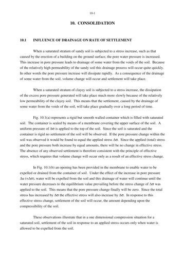
10-26t50 1.95 minSince the sample is drained at both upper and lower boundariesH 17.02 8.5 mmTherefore, the coefficient of consolidation iscv10.8 T50 H2t50 0.197 x 8.521.95 x 60 0.122mm2/sec.OTHER CONSOLIDATION SOLUTIONSIt should be remembered that the Terzaghi consolidation theory discussed above appliesonly to cases of one dimensional drainage in which the parameters cv and mv are constantthroughout the soil layer. Other solutions have been developed for cases where the parameters cvand mv vary with depth; where there is more than one consolidating layer; and where theboundary conditions are such that the drainage is not purely one dimensional (for example seeBiot, 1941 and Gibson and Lumb, 1953).For the case of purely radial drainage under vertical loading of a cylindrical block of soilof diameter D to a central axial drain of diameter d, Barron (1948) has produced a free strainconsolidation solution. The model is illustrated in Fig. 10.13 and the solutions for various valuesof n (D/d) are shown in Fig. 10.14. The time factor (Tr) for radial flow is defined aswhereTr cr t/D2cr radial coefficient of consolidation kr / mv ρw g radial permeabilitykr(10.24)
10-27Fig. 10.14 Consolidation Rates for Radial Flow(after Barron, 1948)Fig. 10.15 Circular Footing, Permeable Top, Permeable Base(after Davis & Poulos, 1972)
10-28For comparative purposes the Terzaghi one dimensional solution for vertical flow hasbeen superimposed on Fig. 10.14 and for this curve the time factor is as defined in section 10.5.Fig. 10.14 may be used for problems in which sand drains are used to accelerate the consolidationof a soil layer which has a high ratio of horizontal to vertical permeability.For evaluating the rate of settlement of circular and strip footings on a soil layer, Davisand Poulos (1972) have produced a number of solutions. Fig. 10.15 gives solutions for a circularfooting on a soil layer with a permeable upper surface and a permeable base. Fig. 10.16 givessolutions for a circular footing on a soil layer with a permeable upper surface and an impermeablebase. Fig. 10.17 gives solutions for a strip footing on a soil layer with a permeable upper surfaceand a permeable base. With these three figures, the time factor (T) is defined aswhereT cv t / h2cv one dimensional coefficient of consolidation for verticalh thickness of soil layer(10.25)drainageThe vertical axis of Figs. 10.15, 10.16 and 10.17 is average degree of pore pressuredissipation (UP). This is calculated on any vertical line and is defined asUP 1- u dz / u dz (10.26)where u and u are as defined in equation (10.15). The degree of pore pressure dissipation (UP)is approximately equal to the degree of settlement (US).
10-29Fig. 10.16 Circular Footing, Permeable Top, Impermeable Base(after Davis & Poulos, 1972)Fig. 10.17 Strip Footing, Permeable Top, Permeable Base (after Davis & Poulos, 1972)
10-30REFERENCESBarron, R.A., (1948), “Consolidation of Fine Grained Soils by Drain Wells”, Trans. ASCE., Vol.113, pp 718-742.Biot, M.A., (1941), “General Theory of Three Dimensional Consolidation”, Jnl. Applied Physics,Vol. 12, pp 155-164.Das, B.M., (1985), “Principles of Geotechnical Engineering”, PWS Publishers, Boston, 571 p.Davis, E.H. and Poulos, H.G., (1972), “Rate of Settlement under Two-and-Three-DimensionalConditions”, Geotechnique Vol. 22, No. 1, pp 95-114.Gibson, R.F. and Lumb, P., (1953), “Numerical Solution of some Problems in the Consolidationof Clay”, Jnl. Instn. Civil Engrs., London, Vol. 2, Part I, pp 182-198.Leonards, G.A. and Girault, P. (1961), “A Study of the One-Dimensional Consolidation Test”,Proc. Fifth Int. Conf.
10-3 is coincident with the ground surface the initial pore pressure u i at any depth z below the ground surface is ui ρw g z the initial total vertical stress σi is σi ρ sat g z and the initial effective vertical stress σ'i is σ'i σi - u i ρ sat g z - ρw g z ρb g z where ρb is the buoyant density of the soil.