Transcription
CS229 Fall 2014, Final Project Report By: Xiao Cai and Ya WangSentiment Analysis on Movie ReviewsIntroductionSentiment Analysis, the process defined as “aims to determine the attitude of a speaker or a writer with respect tosome topic” in Wikipedia, has recently become an active research topic, partly due to its potential use in a widespectrum of applications ranging from “American idol” popularity analysis to product user satisfaction analysis. Withthe rapid growth of online information, a large amount of data is at our fingertips for this kind of analysis. However,the sheer volume of information was a daunting challenge itself. To separate relevant information from the irrelevant,and to gain knowledge from this unprecedented deluge of data, automatic algorithm is essential. In this project, weexplored the use of various supervised machine learning algorithms in learning sentiment classifier and tested theeffectiveness of different feature selection algorithms in improving those classifiers.Input DataThe input data for this project originated from the Rotten Tomatoes dataset: a corpus of movie reviews originallycollected by Pang and Lee [1] for sentiment analysis. According to the information on Kaggle.com where wedownloaded the data, Socher et al. [2] used Amazon's Mechanical Turk to create fine-grained labels for all parsedphrases in the corpus during their work on sentiment treebanks.One pre-labeled training dataset and one unlabeled testing dataset are included. The sentiment labels use integersfrom 0 to 4, with 0 being the most negative and 4 the most positive. The training dataset contains 156,060 datainstances and the testing dataset 66,292. Each data instance comprises attributes: “phrase id”, “sentence id”,“phrase”. The “phrase” attribute contains the actual content of the represented text phrase, which were transformedinto numeric vectors usable by machine learning algorithm using the feature extraction process discussed below.Feature ExtractionFor text analysis, one standard feature extraction approach is to represent text phrases as n-grams, i.e. subsequencesof n words with or without skips. To account for the fact that a word preceded by a negative word such as “barely”has opposite sentiments, we experimented with both unigram and bigram features in this project; the feature vectorsthus produced span a very high dimensional feature space and hence is expected to be very sparse. The special naturemay cause deterministic machine learning algorithms to “overfit”. This issue will be revisited later in the featureselection section.MethodologyNaïve Bayes algorithm, Softmax (Logistic) Regression and Support Vector Machine are all known to be suitable fortext classification but varies in its assumption and formulation of the problem. All were explored in this project.Naïve Bayes Classifier (NBC)As a generative learning algorithm, the Naïve Bayes algorithm models class prior p(y) and conditional feature priorp(x y) from training samples. NB Classifiers learned in this project is based on the multivariate Multinomial eventassumption.Assumption:The multivariate Multinomial event assumes that: given a sentiment of a phrase or data instance , word in oneposition in the phrase tells us nothing about words in other positions; word appearance does not depend on position.Formulas for Prior Estimates: The p(x y) for a feature k is modeled as:of all features appeared in a data instance ;th()() { { ()()}}. Here,denoting the total frequency: the word or more precisely the index of the word at position j ofdata instance ; k: index for the k word in the vocabulary dictionary;m: number of data instances; ( ) : class label for instance . ;V,: vocabulary and its size;
CS229 Fall 2014, Final Project Report By: Xiao Cai and Ya WangThe Laplace smoothing is applied to guarantee that the basic probability axioms: probability being nonnegative andsum to 1, will still hold in the case when a data instance contains an n-gram not found in the dictionary and theestimate without smoothing will otherwise result zero for all sentiment classes. The estimate without the Laplacesmoothing is basically the fraction of times a word k appears across all data instances of label c.{ () The prior p(y) can be modeled as the fraction of data instances with sentiment label c:}.With the priors thus modeled, the Bayes rule is used to derive the posterior distribution on y given x and the classwith highest posterior probability is picked as the prediction of the sentiment class. Give a data instance vectorizedas ( ) * , the mathematical formulation of the predication is as follows:)( ) (()̂()* () ()Softmax (by Stochastic Gradient Descent)Softmax algorithm is another algorithm other than Naïve Bayes, which we implemented using Matlab scriptinglanguage for this project. Unlike Naive Bayes, it belongs to the deterministic algorithm family and aims to learnmappings (using a set of parameters such as below) directly from the input space X to labels y.The model assumes()and *()( ̂) ̂ ()* ( ()̂is its estimate.The Softmax problem of this project is formulated as:()̂( )̂ (̂()The partial gradient of ( ) with respect to( )With(). {()}()( ̂)/())*()()** ())* () can be derived as (due to page limit, no detailed steps are included):()being the parameter for class c and word k;()̂ (): the frequency of word k in data instance ; : vector representing how frequent each word in V appeared in data instance ;Considering that the whole data instances from big data often can‟t be fit in the memory, stochastic gradient descentalgorithm is implemented to solve the parameters for Softmax problem.Initialize to vector of zeros for each label class* Loop through each data instance i { for i 1 to m, {()( )/ ( ) (for each feature k and each label class c). { ()}}}Support Vector MachineSupport Vector machine is another machine algorithm fit for text classification problem for reasons elaborated byJoachims [3]. The implementation of SVM in this project leveraged a third part library: liblinear [4]. The problem isformulated using the standard linear SVM formulation with l1 regularization.,s.t.- ()
CS229 Fall 2014, Final Project Report By: Xiao Cai and Ya WangFeature SelectionRealizing most words in a phrase do not convey sentiments, two feature ranking algorithms are implemented toautomatically identify the corresponding “uninformative” features.Mutual Information (MI) RankMutual Information (MI) index is the feature ranking method related to Naive Bayes algorithm. High MI indicatesthat a feature xi is very “informative” about y. In contrast, a very low MI indicates “non-informative” features.()() ()( ) ( )MI calculated in two different ways are used in this project. One uses the priors modeled in NBC to calculate MI(k,y)for each word k as:() ()()()* Here, () *is the probability of word k appears in phrase i at position j, which based on NB assumption is the same for all data instance i and word position j.The other is to use the formula given in the chapter 13 of Manning‟s book [7]. The same formula as given above canbe used by changing the definition of conditional prior of word k into the following: (){ { ()}(the p(x y) modeled when NB used Multivariate Bernoulli Event assumption).}F-score RankThe F-score is the correlation coefficient between one of the features and the label. It is very similar to F-test statisticsthat measures the difference between variance between different population groups and among each population group.Intuitively, it is a good measure of how “discriminative” a feature is regarding sentiment classes. The formula of Fscore used in this project is a variant of the one used in Chang [5], which instead is for two classes.( ) ( ̅ * () ( )(.̅ )()̅( )/{ ()}), with ̅( ) ()* ()* () and ̅ () Results, Discussion and ConclusionThe models trained using algorithms discussed above are evaluated on both the training data and the test data set. Theprediction for the test data set is scored online by kaggle.com. In the following, some interesting results are presentedand interpreted.Table 1: Comparison of Prediction AccuracyUnigram FeaturesNBCBigram 20%59.20%59.20%Table 1 compares the use of unigram vs bigram and the use of three aforementioned algorithms. On the training data,SoftMax has the best performance and achieves almost perfect predicting accuracy whether using unigram or bigramfeatures; SVM achieved almost perfect prediction accuracy when using bigram. However, NBC consistently beat theother two algorithms on the test data in terms of prediction accuracy. The phenomena can be explained by Vaponic
CS229 Fall 2014, Final Project Report By: Xiao Cai and Ya WangChervonenkis (VC) dimension analysis. The hypothesis function for Softmax use V * C ( V : number features; C :number of classes) number of parameters; while the hypothesis for SVM uses V *( C -1) number of parameters, sinceeach set of parameters that defines a hyper-plane to separate one class from the rest uses has V dimension. Moreparameters for linear or generalized linear models like Softmax (the decision boundary for Softmax is essentiallinear.) and SVM translate into a hypothesis space with higher VC dimension, which itself translates into higher upperbound on the discrepancy between the hypothesis error and the true error, or “overfitting” on testing data. This is onecause which contributes to better performance of Softmax over SVM on training data and overfitting of both on testdata. On the other hand, the higher dimensional space resulted from Bigram renders features vectors sparser andhence higher chances to be separable, which contributed to the improved prediction accuracy of SVM on the trainingdata in the case with Bigram in comparison to the Unigram case. Naïve Bayes, on the other hand, is a generativemodel, which is not as susceptible to the curse of VC dimension or “overfitting”. Instead, according to central limittheorem, the empirical probability based NBC tends to become quite accurate with a large number of data instances.However, the more rigorous assumption of NBC also makes it less accurate in modeling the training data.Figure 1: Prediction Accuracy of NBC and SVM vs. Number of Features80%Top 100Top 1000Top 5000Top 10000All Features70%60%50%40%NBC UnigramModel TrainingNBC UnigramModel TestingNBC BigramModel TrainingNBC BigramModel TestingSVM (Unigram) SVM (Unigram)TrainingTestingFigure 1 illustrates the effectiveness of feature selection by MI index for NBC and by F-score for SVM. It shows thatthe top 1000 features turn out to do an almost as good job as 10,000 features. In addition, the prediction accuracydoesn‟t improve proportionally with the increase in features included in the model. The larger the number of featuresalready included the smaller the improvement in accuracy by adding more features. On the test data, the modelsometimes performs better after irrelevant features had already been tossed out but still having enough relevantfeatures kept.Table 1: Most Informative vs Least Informative by Feature RankNBC Features Ranked by MI5 most informative5 most relish'SVM Features Ranked by F-score5 most informative5 least buddy‟Note 1: The MI shown here is calculated using the formula given in the chapter 13 of Manning’s book [7].Top 5 SVM tokens in order based on F rank turned out to be quite interesting. The top informative token “flopped”unambiguously conveys negative feeling. While the top least informative token “henry” is a name; names usuallydon‟t convey any feeling unless it happens to be something like “Voldemort”. On the contrary, the result of featureranked by MI doesn‟t seem to be as intuitive. After some investigation, we found out that the high MI rank forsentiment neutral words like “goose” and “adage” is due to the fact that these words seem to concentrate in thephrases with class label 2. Hence, MI algorithm identified those as very informative about class label 2, whichhappens to represent neutral sentiment and also constitutes the largest proportion of the document. This inspired thethought that maybe a modified MI ranking which identifies features most informative about the four more extremesentiments could have served a better job. Due to time limitation, the idea is not pursued further in this project.
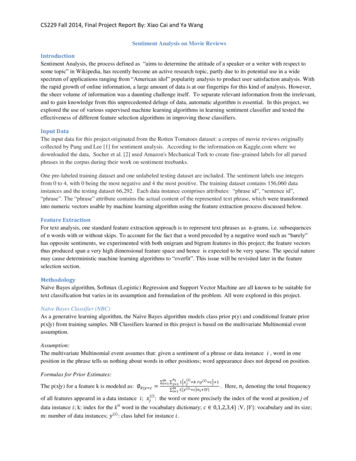
CS229 Fall 2014, Final Project Report By: Xiao Cai and Ya WangNorm(theta(n)-theta(n-1)Figure 2: Convergence of SoftMax Parameters with Passes of Data with learning rate 0.5.The Convergence of Theta for .133450.0901267PassesFigure 2 shows the convergence rate of SoftMax parameters with the number of passes through the training data using0.5 as the learning rate and with 10,000 top features selected using F-score. Though the algorithm converges quickly,due to the large number of data instances, each pass takes a long time to finish. In this aspect, the SoftMax is the leastefficient among the three algorithms tested.The feature selection using F-score turns out to work well for SoftMax algorithm. The model with the top 10,000unigram features achieves a 44.85% accuracy rate on the test data which is better than the accuracy rate 40.95%shown in table 1 for Softmax Model using all features. The model with the top 5000 features resulted 40% accuracyrate on the test data, which is almost the same as the model using all features.In conclusion, through this project, we learned that the deterministic algorithms like SoftMax and SVM is liable toover-fitting in a high dimensional feature space. On the other hand, with its relative rigorous assumption ofconditional independence of features, Naïve Bayes algorithm doesn‟t perform too well on the training data but alsohas less problem of over-fitting. Furthermore, feature selection methods can improve performance and the topfeatures identified by different feature selection methods could differ.Future work:In the future, other feature selection methods or hybrid of feature selection methods will be explored, for instancecombining the top features from the MI ranking with those from F-score ranking. In addition, More sophisticated textanalysis algorithms, such as MaxEm or deep learning/neural network or others will be implemented.Reference:[1] Pang and L. Lee. 2005. Seeing stars: Exploiting class relationships for sentiment categorization with respect torating scales. In ACL, pages 115–124.[2] Recursive Deep Models for Semantic Compositionality Over a Sentiment Treebank, Richard Socher, AlexPerelygin, Jean Wu, Jason Chuang, Chris Manning, Andrew Ng and Chris Potts. Conference on Empirical Methods inNatural Language Processing (EMNLP 2013).[3] Thorsten Joachims, “Text Categorization with Support Vector Machines: Learning with Many Relevant blications/joachims 98a.pdf[4] http://www.csie.ntu.edu.tw/ cjlin/papers/libsvm.pdf[5] Yin-Wen Chang and Chih-Jen Lin, “Feature Ranking using linear SVM”http://www.csie.ntu.edu.tw/ cjlin/papers/causality.pdf[6] Andrew Ng, Stanford CS229 Course Notes, http://cs229.stanford.edu/materials.html[7] Christopher D. Manning, Prabhakar Raghavan, and Hinrich Schütze. 2008.Introduction to Information Retrieval.Cambridge University Press.
phrases in the corpus during their work on sentiment treebanks. One pre-labeled training dataset and one unlabeled testing dataset are included. The sentiment labels use integers from 0 to 4, with 0 being the most negative and 4 the most positive. The training dataset contai