Transcription
Final Report - Application of Machine Learning toAircraft Conceptual DesignAnil VariyarStanford University, CA 94305, U.S.A.I.IntroductionConceptual design and performance estimation for aircraft is a complex multi-disciplinary problem thatinvolves modelling the effects of the aerodynamics, propulsion, stability and structural response of the aircraftfor a speciifed design mission. However, for applications like simulation of the flights across the entire airspaceas shown in Fig 1, it becomes necessary to model tens of thousands of aircraft simultaneously making theproblem extremely computationally expensive. The goal of this project is to use aircraft performance datato build surrogate models using different regression techniques and observe which techniques are best suitedfor the problem at hand. Once the surrogate is build, aircraft missions can be inexpensively simulatedusing the surrogate thus allowing us to solve extremely large design problems involving thousands of designsinexpensively.Figure 1. Air traffic around the world at any instant in timeII.Data and FeaturesThe data used for this problem was obtained by performing simulations on a large number of aircraftof different sizes using a conceptual design code called the Program for Aircraft Synthesis Studies. Thesesimulation were performed a few months ago as part of a research project with the Federal Aviation Administration (FAA). The data set contains the performance estimates of about 48,000 different aircraftconfigurations at different flight conditions. Each data point originally contained 24 inputs and 8 outputs.Of the outputs we are only interested in fuel burn for this project. Moreover, the input dimension is reducedto 7 as described in section A. The 7 inputs (columns) that are fed into the different regression models arethe aircraft payload, the mission range, the takeoff weight, cruise Mach number, wing span, wing sweep andthe wing area. Each of these variables is non- dimensionalised to ensure that they remain between 0 and 1.Table 1 shows a sample data point from the training data set. The data is used to create 6 training sets ofsizes 500, 1000, 2000, 5000, 10000 and 20000 samples and 4 test sets each with 4000 samples.1 of 5American Institute of Aeronautics and Astronautics
A.Feature selectionSequential feature selection is used to reduce the input space from 24 to 7 dimensions. The ’sequentialfs’function in matlab is used for this. It sequentially adds features to an empty set such that they best predicty. The sum of the squared error based on linear regression is used to evaluate the quality of the feature onthe training set. Based on this the 7 input dimensions shown in the table 1 are selected.Table 1. Aircraft ight a (f t2 )1344wingsweep (deg)25Fuel burn(kg)27800ModelsThe different regression models applied to the dataset are described below.Linear RegressionLinear regression was the first algorithm tried. The normal equations θ (X T X) 1 X T y are solved forthe training inputs x and outputs y. θ was then used to compute the outputs for the test data usingytest θ0 θ1 x1 θ2 x2 . The linear regression models seems to work well on the test data. However, theresults are not as accurate as required for the prediction of fuel burn. Moreover as the number of samplesare increased, the error does not improve the estimate by much.Weighted Linear Regression2test ). TheNext weighted linear regression is tried on the data with a weighing function exp ( x x2τ 2modified normal equations solved for this case are θ (X T W X) 1 X T W T y This model doesn’t work muchbetter than the linear regression and is more expensive to compute than linear regression. It also follows atrend similar to linear regression.Higher Order RegressionNow we look at quadratic regression where we use the formula ytest θ0 θ1 x1 θ2 x2 θ3 x1 x2 θ4 x21 θ5 x22 . Addition of the higher dimensional features improves the fit to the training data and reduces the testerror as show in Fig 2. However like the linear and weighted linear regression cases, increasing the numberof samples does not significantly improve the test error.Figure 2. Comparison of linear, weighted linear and quadratic regression2 of 5American Institute of Aeronautics and Astronautics
k-Nearest Neighbours RegressionIn this method, the k- nearest neighbours of the test point are computed and then the estimate of thefuel burnPat the test point is obtained using a weighted average of the values at the k nearest pointskyeval i 1W (i)ytrain (i)Pki 1W (i). We use the inverse of the euclidean distance between the training point i andevaluation point as the weight W (i). The ’knnsearch’ function in matlab is used to compute the k-nearestneighbours and this is fed into matlab code written for this project that performs the prediction and iterationsto compute optimal k. To compute the optimal k, an iterative procedure is used and the value of k thatminimises the mean squre error over the training set is selected. The effect of varying k on the mean squareerror for the different samples is shown in Fig 3(a). It is observed that although for smaller sample sizes thek-NN algorithm does not perform very well, as the sample sizes are increased, the K-NN algorithm is ableto give a fairly good estimate of the fuel burn.Gaussian Process RegressionGaussian process regression is the next method that is applied to the data set. The reason for trying thisis that in a different study, gaussian process regression was successfully used to build surrogate models foraircraft propulsion systems. Selection of the appropriate mean and covariance functions is a tricky task. Forthis study we try 3 different mean and 4 different covariance functions as shown in table 2 . The isotropicmatern covariance function along with either linear or quadratic mean function are the best performingmodels. Figure 3(b) shows how the different Gaussian models perform on the test sets. The capabilities of’gpml’ an existing matlab code for Gaussian Process Regression suplemented by code written for this projectare leveraged for this study.Table 2. Covariance functionsCovariance functionsIsotropic MaternIsotropic RQIsotropic SEARD SEformula k(x , x ) sf 2 f ( d r) e d rpwhere r is ((xp xq )T (P ) 1 (xp xq )),P is a diagonal matrix of the hyperparametersand sf 2 is the signal variancek(xp , xq ) sf 2 [1 (xp xq )T (P ) 1 (xp xq )/(2 α)] αwhere P is the diagonal matrix of the hyperparameters,sf 2 is the signal variance andα is the shape parameterpq T 1pqk(xp , xq ) sf 2 e (x x ) P (x x )/2where P is the diagonal matrix of the hyperparameters,sf 2 is the signal varianceand x is the matrix of input datapqk(x , x ) sf 2 exp (xp xq )T P 1 (xp xq )/2where P is a diagonal matrix with the ARD parameters,sf 2 is the signal variance,x is the matrix of training inputspqwhere RQ stands for Rational Quadratic covariance function SE stands for Squared Exponential covariance function and ARD stands for Automatic Relevance Detemination which is a distance measure3 of 5American Institute of Aeronautics and Astronautics
(a) Effect of varying k for k-NN regression.(b) Comparision of different mean and covariance functionsfor GPR.Figure 3. Plots for k-NN and GPR.Artificial Neural Network - Multilayer Perceptron NetworkA feed-forward Multilayer Perceptron Network is the last method that has been applied to the data.Work done by Bryan Yukto3 as part of his dissertation at MIT has shown that feed forward ANNs providepromising results for prediction of aircraft parameters. We use a 3 layer network with 7 input neuron, 7hidden neurons and 1 output neuron. The network used was arrived at by trying out different 3 and 4 layernetworks by varying the number of hidden layers and neurons in these layers. We try both the sigmoid andthe hyperbolic tangent activation functions. For this study the tanh activation function performs better.Morever, standard gradient descent based back propogation is unable to bring down the training error.Thus a Levenberg Marquardt back propogation error is used for this study. In this method, the gradient gis estimated using J T e where J is the jacobian matrix computed using back propogation as shown in thereferences 1 and e is the error vector for the n training samples. The Hessian H is approximated usingJ T J νI . The weights are then updated using W : W H 1 g. Figure 4 shows the convergence historyof the network for the case with 1000 training samples. For the current study, we stop the training at 10000iterations(as the error is already significantly low. ANN’s are promising for the curent application as thetraining and test error can be significantly reduced even further by training for larger number of iterationsas shown by the trends. A python implementation of the multi-layer perceptron network algorithm alongwith the different back-propogation methods was written from scratch for this project.Figure 4. Convergence of the the Levenberg Marquardt based back propogation4 of 5American Institute of Aeronautics and Astronautics
IV.Summary of the resultsWe summarise the results described in the previous section by tabulating the testing and training errorobtained using the different methods in table 3. The test error stated below are averaged values over the 4test sets of 4000 samples each, for the training set of 1000 samples .Table 3. Comparision of different regression methodsModelTraining MSETest MSELinear RegressionWeighted linear regressionQuadratic Regressionk-NN regressionGaussian Process Regression(best case)Multilayer Perceptron .97e-43.40e-47.84e-41.97e-43.97e-4V.ConclusionWe see that machine learning techniques perform well in predicting aircraft performance. GaussianProcess regression and Artificial Neural Networks are the most promising methods. GPR allows us to reducethe prediction errors significantly and the approximation improves as the number of samples is increased.ANN’s also perform well and importantly as the number of training iterations are increased, the predictionerror can be reduced further. This is encouraging as now, millions of predictions can be performed in amatter of seconds without resorting to parallel computation. This will allow designer to simulate large scaleaircraft systems like the National Airspace system accurately and perform optimizations on air transportationnetworks (changing flight paths and schedules) to try and minimize the overall fuel burn of the system withoutworrying about computational costs.Another interesting trend that jumps out is that simple methods like linear or quadratic regression alsowork fairly well with estimation errors below 5%. This is encouraging as these methods can be used by peoplewith minimal machine learning experience in cases where quick estimates are required, without having toworry about the complications of GPR or ANNs.VI.Future WorkThe studies for this case were all performed on conventional aircraft configurations. Looking to see if thesemethods work for unconcentional aircraft configurations like Blended wing bodies etc. will be an interestingnext step. For those configurations, the interactions between the different disciplines are extremely complexand modelling them using regression methods might not work out as well as they did for this case.References1 Hao,Y. and Wilamowski, B.M,“Levenberg-Marquardt Training,” , notes.C.E. and Williams, C.K.I, “Gaussian Processes for Machine Learning,” , The MIT Press, 2006. ISBN 0-262-2 Rasmussen,18253-X.3 Yukto, B, ”The Impact of Aircraft Design Reference Mission on fuel Efficiency in the Air Transportation System” , PhDThesis, MIT Aero Astro4 Ebden, M., “Gaussian Processes for Regression,” ,notes.5 Hagan, M.T. and Menhaj. M.B, “Training Feedforward Networks with Marquardt Algorithm,” IEEE Transactions onNeural Networks, Vol. 5 No. 6, NOvember 1996 .5 of 5American Institute of Aeronautics and Astronautics
Final Report - Application of Machine Learning to Aircraft Conceptual Design Anil Variyar Stanford University, CA 94305, U.S.A. I. Introduction Conceptual design and performance estimation