Transcription
10.1098/rsta.2003.1190Self-organizing neural systemsbased on predictive learningBy R a j e s h P. N. R a o1 a n d T e r r e n c e J. Sejnowski2,31Department of Computer Science and Engineering, University of Washington,Box 352350, Seattle, WA 98195-2350, USA (rao@cs.washington.edu)2Computational Neurobiology Laboratory, Howard Hughes Medical Institute,The Salk Institute for Biological Studies, La Jolla, CA 92037, USA3Department of Biology, University of California at San Diego,La Jolla, CA 92037, USA (terry@salk.edu)Published online 6 May 2003The ability to predict future events based on the past is an important attribute oforganisms that engage in adaptive behaviour. One prominent computational methodfor learning to predict is called temporal-difference (TD) learning. It is so namedbecause it uses the difference between successive predictions to learn to predict correctly. TD learning is well suited to modelling the biological phenomenon of conditioning, wherein an organism learns to predict a reward even though the reward mayoccur later in time. We review a model for conditioning in bees based on TD learning.The model illustrates how the TD-learning algorithm allows an organism to learn anappropriate sequence of actions leading up to a reward, based solely on reinforcementsignals. The second part of the paper describes how TD learning can be used at thecellular level to model the recently discovered phenomenon of spike-timing-dependentplasticity. Using a biophysical model of a neocortical neuron, we demonstrate thatthe shape of the spike-timing-dependent learning windows found in biology can beinterpreted as a form of TD learning occurring at the cellular level. We conclude byshowing that such spike-based TD-learning mechanisms can produce direction selectivity in visual-motion-sensitive cells and can endow recurrent neocortical circuitswith the powerful ability to predict their inputs at the millisecond time-scale.Keywords: neuroscience; cerebral cortex; conditioning;synaptic plasticity; visual perception; prediction1. IntroductionLearning and predicting temporal sequences from experience underlies much of adaptive behaviour in both animals and machines. The smell of freshly baked bread maybring to mind the image of a loaf; the unexpected ring of a doorbell may promptthoughts of a salesperson at the door; the disappearance of a car behind a slow moving bus elicits an expectation of the car’s reappearance after an appropriate delay;the initial notes from an oft-repeated Beatles song prompts a recall of the entire song.These examples illustrate the ubiquitous nature of prediction in behaviour. Our ability to predict depends crucially on the statistical regularities that characterize theOne contribution of 18 to a Theme ‘Self-organization: the quest for the origin and evolution of structure’.Phil. Trans. R. Soc. Lond. A (2003) 361, 1149–11751149c 2003 The Royal Society
1150R. P. N. Rao and T. J. Sejnowskinatural world (Atick & Redlich 1992; Barlow 1961; Bell & Sejnowski 1997; Dong &Atick 1995; Eckert & Buchsbaum 1993; MacKay 1956; Olshausen & Field 1996; Rao1999; Rao & Ballard 1997, 1999; Schwartz & Simoncelli 2001). Indeed, predictionwould be impossible in a world that is statistically random.The role of prediction in behavioural learning was investigated in early psychological experiments by Pavlov and others (see Rescorla (1988) for a review). In thefamous Pavlovian conditioning experiments, a dog learned to salivate when a bellwas rung, after a training session in which an appetizing food stimulus was presentedright after the bell. The dog thus learned to predict a food reward (the unconditionedstimulus) based on a hitherto unrelated auditory stimulus (the conditioned stimulus).Several major areas in the brain have been implicated in the learning of rewards andpunishments, such as the dopaminergic system, the amygdala, and the cerebellum.At a more general level, it has been suggested that one of the dominant functions ofthe neocortex is prediction and sequence learning (Barlow 1998; MacKay 1956; Rao1999; Rao & Ballard 1997, 1999).A major challenge from a computational point of view is to devise algorithmsfor prediction and sequence learning that rely solely on interactions with the environment. Several approaches have been suggested, especially in control theory andengineering, such as Kalman filtering, hidden Markov models, and dynamic Bayesiannetworks (see Ghahramani (2001) for a review). A popular algorithm for learningto predict is temporal-difference (TD) learning (Sutton 1988). TD learning was proposed by Sutton as an ‘on-line’ algorithm for reinforcement-based learning, whereinan agent is given a scalar reward typically after the completion of a sequence ofactions that lead to a desired goal state. The TD-learning algorithm has been enormously influential in the machine learning community, with a wide variety of applications, having even produced a world-class backgammon playing program (Tesauro1989). We review the basic TD-learning model in § 2.TD learning has been used to model the phenomenon of conditioning wherein ananimal learns to predict a reward based on past stimuli. Sutton & Barto (1990)studied a TD-learning model of classical conditioning. Montague et al . (1995) haveapplied TD learning to the problem of reinforcement learning in foraging bees. Thereis also evidence for physiological signals in the primate brain that resemble theprediction error seen in TD learning (Schultz et al . 1997). We review some of theseresults in §§ 2 and 3.The idea of learning to predict based on the temporal difference of successivepredictions can also be applied to learning at the cellular level (Dayan 2002; Rao &Sejnowski 2000, 2001). In § 4, we link TD learning to spike-timing-dependent synapticplasticity (Bi & Poo 1998; Gerstner et al . 1996; Levy & Steward 1983; Markram et al .1997; Sejnowski 1999; Zhang et al . 1998) and review simulation results. We show thatspike-based TD learning causes neurons to become direction selective when exposedto moving visual stimuli. Our results suggest that spike-based TD learning is a powerful mechanism for prediction and sequence learning in recurrent neocortical circuits.2. Temporal-difference learningTD learning is a popular computational algorithm for learning to predict inputs(Montague & Sejnowski 1994; Sutton 1988). Learning takes place based on whetherthe difference between two temporally separated predictions is positive or negative.Phil. Trans. R. Soc. Lond. A (2003)
Self-organizing neural systems1151This minimizes the errors in prediction by ensuring that the prediction generatedafter adapting the parameters (for example, the synapses of a neuron) is closer tothe desired value than before.The simplest example of a TD-learning rule arises in the problem of predicting ascalar quantity z using a neuron with synaptic weights w(1), . . . , w(k) (representedas a vector w). The neuron receives as presynaptic input the sequence of vectorsx1 , . . . , xm . The output of the neuron at time t is assumed to be given by Pt i w(i)xt (i). The goal is to learn a set of synaptic weights such that the predictionPt is as close as possible to the target z. According to the temporal-difference (TD(0))learning rule (Sutton 1988), the weights at time t 1 are given bywt 1 wt λ(Pt 1 Pt )xt ,(2.1)where λ is a learning rate or gain parameter and the last value of P is set to thetarget value, i.e. Pm 1 z. Note that learning is governed by the temporal differencein the outputs at time instants t 1 and t in conjunction with the input xt at time t.To understand the rationale behind the simple TD-learning rule, consider thecase where all the weights are initially zero, which yields a prediction Pt 0 forall t. However, in the last time-step t m, there is a non-zero prediction error(Pm 1 Pm ) (z 0) z. Given that the prediction error is z at the last time-step,the weights are changed by an amount equal to λzxt . Thus, in the next trial, theprediction Pm will be closer to z than before, and after several trials, will tend toconverge to z. The striking feature of the TD algorithm is that, because Pm actsas a training signal for Pm 1 , which in turn acts as a training signal for Pm 2 andso on, information about the target z is propagated backwards in time such thatthe predictions Pt at all previous time-steps are corrected over many trials and willeventually converge to the target z, even though the target only occurs at the endof the trial.One way of to interpret z is to view it as the reward delivered to an animal at theend of a trial. We can generalize this idea by assuming that a reward rt is deliveredat each time-step t, where rt could potentially be zero. As Sutton & Barto (1990)originally suggested, the phenomenon of conditioning in animals can be modelled asthe prediction mtime m of the sum of future rewards in a trial, starting from the currentstep t: i t ri . In other words, we want Pt i w(i)xt (i) to approximate i t ri .Note that, ideally,Pt m ri rt 1 i tm ri rt 1 Pt 1 .(2.2)i t 1Therefore, the error in prediction is given byδt rt 1 Pt 1 Pt(2.3)and the weights can be updated as follows to minimize the prediction error:wt 1 wt λ(rt 1 Pt 1 Pt )xt .(2.4)This equation implements the standard TD-learning rule (also known as TD(0))(Sutton 1988; Sutton & Barto 1998). Note that it depends on both the immediatereward rt 1 and the temporal difference between the predictions at time t 1 and t.Phil. Trans. R. Soc. Lond. A (2003)
1152R. P. N. Rao and T. J. SejnowskiConsiderable theory exists to show that the rule and its variants converge to thecorrect values under appropriate circumstances (see Sutton & Barto 1998).Beginning with Sutton & Barto’s early work on TD learning as a model for classical conditioning, a number of researchers have used TD learning to explain bothbehavioural and neural data. One important application of TD learning has beenin interpreting the transient activity of cells in the dopamine system of primates:the activity of many of these cells (for example, in the ventral tegmental area) isstrikingly similar to the temporal-difference error δt that would be expected duringthe course of learning to predict rewards in a particular task (Schultz et al . 1995,1997). Another demonstration of the utility of the TD-learning algorithm has beenin modelling foraging behaviour in bees. Results from this study are reviewed in thenext section.3. TD-learning model of conditioning in beesIn addition to the sensory and motor systems that guide the behaviour of vertebrates and invertebrates, all species also have a set of small nuclei that projectaxons throughout the brain and release neurotransmitters such as dopamine, norepinephrine, and acetylcholine (Morrison & Magistretti 1983). The activity in someof these systems may report on expectation of future reward (Cole & Robbins 1992;Schultz et al . 1995, 1997; Wise 1982). For example, honeybees can be conditioned toa sensory stimulus such as colour, shape or smell of a flower when paired with application of sucrose to the antennae or proboscis. An identified neuron, VUMmx1, projectswidely throughout the entire bee brain, becomes active in response to sucrose, and itsfiring can substitute for the unconditioned odour stimulus in classical conditioningexperiments. A simple model based on TD learning can explain many properties ofbee foraging (Montague et al . 1994, 1995).Real and co-workers (Real 1991; Real et al . 1990) performed a series of experiments on bumble bees foraging on artificial flowers whose colours, blue and yellow,predicted the delivery of nectar. They examined how bees respond to the mean andvariability of this delivery in a foraging version of a stochastic two-armed-banditproblem (Berry & Fristedt 1985). All the blue flowers contained 2 µl of nectar, 13 ofthe yellow flowers contained 6 µl, and the remaining 23 of the yellow flowers containedno nectar at all. In practice, 85% of the bees’ visits were to the constant-yield blueflowers despite the equivalent mean return from the more variable yellow flowers.When the contingencies for reward were reversed, the bees switched their preferencefor flower colour within one to three visits to flowers. Real and co-workers furtherdemonstrated that the bees could be induced to visit the variable and constant flowers with equal frequency if the mean reward from the variable flower type was madesufficiently high.This experimental finding shows that bumble bees, like honeybees, can learn toassociate colour with reward. Further, colour and odour learning in honeybees hasapproximately the same time course as the shift in preference described above for thebumble bees (Gould 1987). It also indicates that under the conditions of a foragingtask, bees prefer less variable rewards and compute the reward availability in theshort term. This is a behavioural strategy used by a variety of animals under similarconditions for reward (Krebs et al . 1978; Real 1991; Real et al . 1990), suggesting acommon set of constraints in the underlying neural substrate.Phil. Trans. R. Soc. Lond. A (2003)
Self-organizing neural systemsnectarS1153sensory inputBYaction igure 1. Neural architecture of the bee-foraging model. During bee foraging (Real 1991), sensoryinput drives the units B and Y representing blue and yellow flowers. These units project toa reinforcement neuron P through a set of variable weights (filled circles wB and wY ) andto an action selection system. Unit S provides input to R and fires while the bee sips thenectar. R projects its output rt through a fixed weight to P . The variable weights onto Pimplement predictions about future reward rt (see text) and P ’s output is sensitive to temporalchanges in its input. The output projections of P , δt (lines with arrows), influence learningand also the selection of actions such as steering in flight and landing, as in equation (3.2)(see text). Modulated lateral inhibition (dark circle) in the action selection layer symbolizesthis. Before encountering a flower and its nectar, the output of P will reflect the temporaldifference only between the sensory inputs B and Y . During an encounter with a flower andnectar, the prediction error δt is determined by the output of B or Y and R, and learning occursat connections wB and wY . These strengths are modified according to the correlation betweenpresynaptic activity and the prediction error δt produced by neuron P as in equation (3.1) (seetext). Learning is restricted to visits to flowers. (Adapted from Montague et al . (1994).)Figure 1 shows a diagram of the model architecture, which is based on the anatomyand physiological properties of VUMmx1. Sensory input drives the units ‘B’ and ‘Y ’Yrepresenting blue and yellow flowers. These neurons (outputs xBt and xt , respectively,at time t) project through excitatory connection weights both to a diffusely projectingneuron P (weights wB and wY ) and to other processing stages which control theselection of actions such as steering in flight and landing. P receives additional inputrt through unchangeable weights. In the absence of nectar (rt 0), the net input toY YP becomes Pt wt · xt wtB xBt wt xt .Assume that the firing rate of P is sensitive only to changes in its input overtime and habituates to constant or slowly varying input. Under this assumption, theerror in prediction is given by δt in equation (2.3), and the weights can be updatedaccording to the TD-learning rule in equation (2.4). This permits the weights ontoP to act as predictions of the expected reward consequent on landing on a flower.When the bee actually lands on a flower and samples the nectar, R influences theoutput of P through its fixed connection (figure 1). Suppose that just prior to sampling the nectar the bee switched to viewing a blue flower, for example. Then, sinceBBBrt 1 0, δt would be rt xBt 1 wt 1 . In this way, the term xt 1 wt 1 is a prediction ofBBthe value of rt and the difference rt xt 1 wt 1 is the error in that prediction. Adjusting the weight wtB according to the TD rule in equation (2.4) allows the weight wtB ,through P ’s outputs, to report to the rest of the brain the amount of reinforcementrt expected from blue flowers when they are sensed.Phil. Trans. R. Soc. Lond. A (2003)
1154R. P. N. Rao and T. J. SejnowskiAs the model bee flies between flowers, reinforcement from nectar is not present(rt 0) and δt is proportional to Pt Pt 1 . wB and wY can again be used as predictions but through modulation of action choice. For example, suppose the learningprocess in equation (2.4) sets wY less than wB . In flight, switching from viewingyellow flowers to viewing blue flowers causes δt to be positive and biases the activityin any action selection units driven by outgoing connections from B. This makes thebee more likely than chance to land on or steer towards blue flowers.The biological assumptions of this neural architecture are explicit:(i) the diffusely projecting neuron changes its firing according to the temporaldifference in its inputs;(ii) the output of P is used to adjust its weights upon landing; and(iii) the output otherwise biases the selection of actions by modulating the activityof its target neurons.For the particular case of the bee, both the learning rule described in equation (2.4)and the biasing of action selection described above can be further simplified. Significant learning about a particular flower colour only occurs in the 1–2 s just prior to anencounter (Menzel & Erber 1978). This is tantamount to restricting weight changesto each encounter with the reinforcer, which allows only the sensory input just preceding the delivery or non-delivery of rt to drive synaptic plasticity. We thereforemake the learning rule punctate, updating the weights on a flower by flower basis.During each encounter with the reinforcer in the environment, P produces a prediction error δt rt Pt 1 , where rt is the actual reward at time t, and the last flowerBxBcolour seen by the bee at time t, say blue, causes a prediction Pt 1 wt 1t 1 ofBfuture reward rt to be made through the weight wt 1 and the input activity xBt 1 .The weights are then updated using the TD-learning rule,wt wt 1 λδt xt 1 ,(3.1)where λ is the learning rate.We model the temporal biasing of actions such as steering and landing with aprobabilistic algorithm that uses the same weights onto P to choose which flower isactually visited on each trial. At each flower visit, the predictions are used directlyto choose an action, according toQ(Y ) exp(µ(wY xY )),exp(µ(wB xB )) exp(µ(wY xY ))(3.2)where Q(Y ) is the probability of choosing a yellow flower. Values of µ 0 amplifythe difference between the two predictions, so that larger values of µ make it morelikely that the larger prediction will result in choice toward the associated flowercolour. In the limit as µ this approaches a winner-take-all rule.To apply the model to the foraging experiment, it is necessary to specify howthe amount of nectar in a particular flower gets reported to P . We assume that thereinforcement neuron R delivers its signal rt as a saturating function of nectar volume(figure 2a). Harder & Real (1987) suggest just this sort of decelerating function ofnectar volume and justify it on biomechanical grounds. Figure 2b shows the behaviourPhil. Trans. R. Soc. Lond. A (2003)
Self-organizing neural systems1001.0 (a)1155beeλ 0.9λ 0.1λ 0(b)80visits to blue (%)output0.80.60.405nectar volume (µl)100(c)10trial203030 (d)806040v 0v 2v 8v 302002mean46variancevisits to variable type (%)40200.21006020100λ 0.1λ 0.9bee2mean46Figure 2. Simulations of bee foraging behaviour using TD learning. (a) Reinforcement neuronoutput as a function of nectar volume for a fixed concentration of nectar (Real 1991; Real etal . 1990). (b) Proportion of visits to blue flowers. Each trial represents approximately 40 flowervisits averaged over five real bees and exactly 40 flower visits for a single model bee. Trials 1–15for the real and model bees had blue flowers as the constant type; the remaining trials hadyellow flowers as constant. At the beginning of each trial, wY and wB were set to 0.5, whichis consistent with evidence that information from past foraging bouts is not used (Menzel &Erber 1978). The real bees were more variable than the model bees: sources of stochasticitysuch as the two-dimensional feeding ground were not represented. The real bees also had aslight preference for blue flowers (Menzel et al . 1974). Note the slow drop for λ 0.1 when theflowers are switched. (c) Method of selecting indifference points. The indifference point is takenas the first mean for a given variance (v in the legend) for which a stochastic trial demonstratesthe indifference. This method of calculation tends to bias the indifference points to the left.(d) Indifference plot for model and real bees. Each point represents the (mean, variance) pairfor which the bee sampled each flower type equally. The circles are for λ 0.1 and the plusesare for λ 0.9. (Adapted from Montague et al . (1994).)of model bees compared with that of real bees (Real 1991). Further details arepresented in the figure legend.The behaviour of the model matched the observed data for λ 0.9, suggesting thatthe real bee uses information over a small time window for controlling its foraging(Real 1991). At this value of λ, the average proportion of visits to blue was 85%for the real bees and 83% for the model bees. The constant and variable flowertypes were switched at trial 15 and both bees switched flower preference in one toPhil. Trans. R. Soc. Lond. A (2003)
1156R. P. N. Rao and T. J. Sejnowskithree subsequent visits. The average proportion of visits to blue changed to 23%and 20%, respectively, for the real and model bee. Part of the reason for the realbees’ apparent preference for blue may come from inherent biases. Honey bees, forinstance, are known to learn about shorter wavelengths more quickly than others(Menzel et al . 1974). In our model, the learning rate λ is a measure of the length oftime over which an observation exerts an influence on flower selection rather thanbeing a measure of the bee’s time horizon in terms of the mean rate of energy intake(Real 1991; Real et al . 1990).Real bees can be induced to forage equally on the constant and variable flower typesif the mean reward from the variable type is made sufficiently large (figure 2c, d). Fora given variance, the mean reward was increased until the bees appeared to be indifferent between their choice of flowers. In this experiment, the constant flower typecontained 0.5 µl of nectar. The data for the real bee are shown as points connectedby a solid line in order to make clear the envelope of the real data. The indifferencepoints for λ 0.1 (circles) and λ 0.9 (pluses) also demonstrate that a higher valueof λ is again better at reproducing the bee’s behaviour. The model captured boththe functional relationship and the spread of the real data.This model was implemented and tested in several ways. First, a virtual bee wassimulated foraging in a virtual field of coloured flowers. In these simulations, the fieldof view of the bee was updated according to the decision rule above (equation (3.2)),so that the bee eventually ‘landed’ on a virtual flower and the trial was repeated(Montague et al . 1995). In a second test, an actual robot bee was constructed andplaced in the centre of a circular field. The robot bee had a camera that detectedcoloured paper on the walls of the enclosure and moved toward the wall using theabove decision rule (P. Yates, P. R. Montague, P. Dayan & T. J. Sejnowski, unpublished results). In each of these tests, the statistics of flower visits qualitatively confirmed the results shown in figure 2, despite the differences in the dynamics of themodel bees in the two circumstances. This is an important test since the complicatedcontingencies of the real world, such as the slip in the wheels of the robot and randominfluences that are not taken into account in the idealized simulations shown here,did not affect the regularities in the overall behaviour that emerged from the use ofthe TD-learning rule.A similar model has been used to model the primate dopamine pathways that alsomay be involved in the prediction of future reward (Montague et al . 1996; Schultzet al . 1997). In this case, the neurons are located in the ventral tegmental area andproject diffusely through the basal ganglia and the cerebral cortex, particularly to theprefrontal cortex, which is involved in planning actions. Thus, there is a remarkableevolutionary convergence of reward prediction systems in animals as diverse as beesand primates.4. TD learning at the cellular level: spike-timing-dependent plasticityA recently discovered phenomenon in spiking neurons appears to share some of thecharacteristics of TD learning. Known as spike-timing-dependent synaptic plasticityor temporally asymmetric Hebbian learning, the phenomenon captures the influenceof relative timing between input and output spikes in a neuron. Specifically, aninput synapse to a given neuron that is activated slightly before the neuron firesis strengthened, whereas a synapse that is activated slightly after is weakened. ThePhil. Trans. R. Soc. Lond. A (2003)
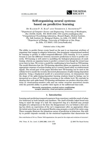
Self-organizing neural systems(b)30 mV(a)1157(c)soma30 mVdendrite3 msFigure 3. Model neuron response properties. (a) Response of a model neuron to a 70 pA currentpulse injection into the soma for 900 ms. (b) Response of the same model neuron to Poisson distributed excitatory and inhibitory synaptic inputs at random locations on the dendrite.(c) Example of a back-propagating action potential in the dendrite of the model neuron as compared with the corresponding action potential in the soma (enlarged from the initial portion ofthe trace in (b)). (From Rao & Sejnowski (2001).)window of plasticity typically ranges from 40 to 40 ms. Such a form of synapticplasticity has been observed in recurrent cortical synapses (Markram et al . 1997), inthe hippocampus (Bi & Poo 1998; Levy & Steward 1983), in the tectum (Zhang etal . 1998), and in layer II/II of rat somatosensory cortex (Feldman 2000).In order to ascertain whether spike-timing-dependent plasticity in cortical neurons can be interpreted as a form of TD learning, we used a two-compartmentmodel of a cortical neuron consisting of a dendrite and a soma-axon compartment(figure 3). The compartmental model was based on a previous study that demonstrated the ability of such a model to reproduce a range of cortical response properties (Mainen & Sejnowski 1996). Four voltage-dependent currents and one calciumdependent current were simulated, as in Mainen & Sejnowski (1996): fast Na , INa ;fast K , IKv ; slow non-inactivating K , IKm ; high voltage-activated Ca2 , ICa andcalcium-dependent K current, IKCa . The following active conductance densities wereused in the soma-axon compartment (in pS µm 2 ): ḡNa 40 000 and ḡKv 1400.For the dendritic compartment, we used the following values: ḡNa 20, ḡCa 0.2,ḡKm 0.1, and ḡKCa 3, with leak conductance 33.3 µS cm 2 and specific membrane resistance 30 kΩ cm 2 . The presence of voltage-activated sodium channels inthe dendrite allowed back propagation of action potentials from the soma into thedendrite as shown in figure 3c.Conventional Hodgkin–Huxley-type kinetics were used for all currents (integrationtime-step, 25 µs; temperature, 37 C). Ionic currents I were calculated using thePhil. Trans. R. Soc. Lond. A (2003)
1158R. P. N. Rao and T. J. Sejnowskiohmic equationI ḡAx B(V E),(4.1)where ḡ is the maximal ionic conductance density, A and B are activation and inactivation variables, respectively (x denotes the order of kinetics; see Mainen & Sejnowski1996), and E is the reversal potential for the given ion species (EK 90 mV,ENa 60 mV, ECa 140 mV, Eleak 70 mV). For all compartments, the specific membrane capacitance was 0.75 µF cm 2 . Two key parameters governing theresponse properties of the model neuron are (Mainen & Sejnowski 1996) the ratio ofaxo-somatic area to dendritic membrane area (ρ) and the coupling resistance betweenthe two compartments (κ). For the present simulations, we used the values ρ 150(with an area of 100 µm2 for the soma-axon compartment) and a coupling resistanceof κ 8 MΩ. Poisson-distributed synaptic inputs to the dendrite (see figure 3b) weresimulated using alpha-function-shaped (Koch 1999) current pulse injections (timeconstant 5 ms) at Poisson intervals with a mean presynaptic firing frequency of 3 Hz.To study plasticity, excitatory postsynaptic potentials (EPSPs) were elicited atdifferent time delays with respect to postsynaptic spiking by presynaptic activationof a single excitatory synapse located on the dendrite. Synaptic currents were calculated using a kinetic model of synaptic transmission with model parameters fitted towhole-cell recorded AMPA (a-amino 3-hydroxy 5-methylisoxazole 4-proprionic acid)currents (see Destexhe et al . (1998) for more details). Synaptic plasticity was simulated by incrementing or decrementing the value for maximal synaptic conductanceby an amount proportional to the temporal difference in the postsynaptic membranepotential at time instants t t and t for presynaptic activation at time t. Thedelay parameter t was set to 10 ms to yield results consistent with previous physiological experiments (Bi & Poo 1998; Markram et al . 1997). Presynaptic input tothe model neuron was paired with postsynaptic spiking by injecting a depolarizingcurrent pulse (10 ms, 200 pA) into the soma. Changes in synaptic efficacy were monitored by applying a test stimulus before and after pairing, and recording the EPSPevoked by the test stimulus.Figure 4 shows the results of pairings in which the postsynaptic spike was triggered5 ms after and 5 ms before the onset of the E
May 06, 2003 · experiments. A simple model based on TD learning can explain many properties of bee foraging (Montague et al. 1994, 1995). Real and co-workers (Real 1991; Real et al. 1990) performed a series of experi-ments on bumble bees foraging on artificial flowers whose co