WIXLIB

Demographic Research: Volume 39, Article 37given age at time t is N (a, t) e ra N (a, t a). Therefore, our basic result (1*) canalso be used to estimate the unknown age structure at initial time t,(6*)c(a, t) e t) r Ne (a, t)e ra N (a, t a)D(a,N (a, t) e ra.N (t)N (t)N (t)It may also be interesting to observe that (6*) is equivalent to a more common expression for the proportion of the population at age a in terms of the birth rate b,(7)c(a, t) b e ra (a),as stated by Lotka more than a century ago (Lotka 1907). Equation (7) implies that thepopulation structure does not depend on time because the birth rate b is constant. Here,we use the notation c(a, t) to highlight that we refer to the age structure at the time ofcapture when the follow-up of the population starts. But in stable populations, the periodage structure – as well as the cohort survival schedule – is constant over time, so onecould simply write c(a).5Although stability is an abstract mathematical concept resulting from the continuous operation of strong demographic assumptions over the long run, these restrictionshave turned out to be serviceable in many applications. Stable population theory hasbeen widely used in the study of human and nonhuman populations, especially when accurate data is incomplete or problematic, as discussed in the manual The Concept of aStable Population: Application to the Study of Populations of Countries with IncompleteDemographic Statistics (United Nations 1968). Even though perfect stability is rarelyobserved, this book argues that many populations around the world are ‘semi-stable’ or‘quasi-stable,’ and possess some of the properties of the stable population model. Semistable refers to populations that have an unchanging age structure, whereas quasi-stabledescribes populations in which fertility remains unchanged and mortality improves gradually.3.2 Life lived and left in stationary populationsIn stationary populations, in addition to fixed age-specific death rates and closure to migration, the birth flow is constant over time because of the growth rate r 0, whichimplies that, in the long run, the number of births equals the number of deaths and thepopulation size remains constant. This approach is more restrictive than stability but canlead to new insights about population dynamics. Some of these insights pertain to thesymmetries between life lived and life left. Kim and Aron (1989) – and later Goldstein5 For a general overview of the main properties of stable populations, see for instance Preston, Heuveline, andGuillot (2001, Chapter 7).http://www.demographic-research.org995

Vaupel & Villavicencio: Estimating age-specific survival in stable populations with unknown ages(2009) – proved that the average age of a stationary population equals average remaining life expectancy, whereas Riffe (2015) addressed the equivalence between the force ofmortality by age and the force of increment by life left. Moreover, stationary populationspresent a symmetry between their age composition and the distribution of remaining lifetimes. This relationship was first described by Brouard (1986, 1989), and was later independently formulated by James Carey and colleagues in the study of the survival patternsof captive and follow-up cohorts of medflies (Müller et al. 2004, 2007). Vaupel (2009)proved that in stationary populations of infinite size and in continuous time, the probability that a randomly selected individual is age a equals the probability that an individualhas exactly a time left until death. Villavicencio and Riffe (2016) suggested an alternativeproof for empirical and finite stationary populations in a discrete-time framework.An alternative perspective is to consider the births and deaths in stationary populations, which need to be continuously in balance to keep the population size constant.Hence, the number of individuals at age 0 (births) equals the number of individuals with0 life left (deaths). Note that the first group forms a birth cohort, whereas in the secondthere are individuals from different ages who share the same time of death, forming a‘death cohort.’ The key point is that this result is true for all ages when the populationis stationary, meaning that the number of individuals at any age a equals the number ofindividuals with a life left within the population. Figure 1 illustrates these ideas: Life leftis plotted in the negative horizontal axis to convey the notion of a ‘countdown.’Figure 1:Symmetries between the age composition and the distribution ofremaining lifetimes in stationary populationsagedistributiondistribution ofremaininglifetimes ω a2 a10life lefta1a2ωage / life livedNote: Parameter ω refers to the maximum observed lifespan.Equation (1*) extends this result to stable populations, so it can be used with lessrestrictive assumptions. In this case there is not an exact symmetry between life lived996http://www.demographic-research.org

Demographic Research: Volume 39, Article 37and left because of the growth rate r, but there is still a relationship between the agecomposition (captured by N (a, t)) and the distribution of remaining lifetimes (capturede t)). Note that if r 0, then N (a, t a) N (a, t) and (1*) becomesby D(a,e t).N (a, t) D(a,This equivalence formalizes the concept of symmetry between life lived and left in stationary populations that has just been described: The number of individuals aged a attime t equals the number of individuals who will die at time t a.3.3 The population of France from a life left perspectiveBrouard (1986) presents an original overview of the population dynamics of France in the20th century from a life left perspective. He compares the age structure of the French population in several years with what he calls the ‘pyramide des années à vivre,’ that is, theprojected structure of remaining lifetimes of the cohorts alive in those years. He also introduces the concept of ‘génération de décès’ (death cohort) mentioned above. Especiallyrelevant are the two pyramids from 1901, which show that the male population above age70 is surprisingly close to the population that at that time had more than 70 years of lifeleft and lived at least until 1970. Lower remaining lifetimes were caused by traumaticevents such as the two world wars that increased mortality, but in general there is a fairlyclose symmetry between both pyramids. In contrast, in the case of women the improvements in mortality were more marked, and thus the pyramid of remaining lifetimes hasmore individuals with higher values, given that more women lived longer than 70 yearsafter 1901 than those above age 70 in that year. Brouard concludes that the analysis ofthe remaining lifetimes offers a new interesting perspective for the study of populationdynamics, notably for older ages. He suggests the estimation of life left according tosome health markers, which could provide better insights into the characteristics of theold population and help in the assessment of proper policies.4. ApplicationDemographers like to think of time as a continuous process, which permits the use ofdifferential calculus and facilitates the proof of demographic relationships among demographic functions. This has been the case in the statement and proof of (1*) and (2*), aswell in the works mentioned above that are based on the stable population theory developed by Lotka (1939).In a theoretical population model, it is reasonable to assume time to be continuous, and compute vital rates and the instantaneous – although theoretical and potentiallyhttp://www.demographic-research.org997

Vaupel & Villavicencio: Estimating age-specific survival in stable populations with unknown agesnoninteger – number of births and deaths at any time. On the contrary, in an empiricalpopulation in which individuals are indivisible, the instantaneous number of births anddeaths would be zero, and the number of births and deaths would have to be computedin time intervals between observations. Villavicencio and Riffe (2016) adopted this approach to provide an alternative proof of the symmetries between life lived and left inempirical stationary populations. This approach represents a more realistic setup, but hasthe disadvantage of making the demonstration more complex than in the continuous case.4.1 Life lived and left in a discrete-time frameworkIn an empirical setup, some adjustments are necessary to adapt Equations (1*), (2*),and (6*) to a discrete-time framework. In general, we can only get the population countsat exact times t, t 1, t 2, etc., and we may not be able to know what births and deathsoccurred between observations. Moreover, a slightly different notation is usually adoptedto account for the fact that ages are not exact: In the following, we use subindices for theage variable to refer to the ‘age interval [a, a 1)’ instead of the ‘exact age a.’Suppose a population is first captured at time t and the total number of individualsN (t) is recorded. This same population is observed again at time t 1 and the numbere1 (t), the individuals from the initialof individuals still alive are recorded, obtaining Npopulation who are alive at time t 1, all of them at age 1 and above. The assumption ofstability implies(8)e1 (t),N1 (t) e r Nwhere N1 (t) is the unknown number of individuals that at exact time t were age 1 andabove. Equation (8) can be used to estimate the population at age [0, 1) at exact time t:N0 (t) N (t) N1 (t)e0 (t) e r Ne1 (t), Ne0 (t), the population at age 0 and above at exact time t. Analogously,given that N (t) Ne1 (t) N2 (t 1)N1 (t 1) Ne1 (t) e r Ne2 (t), Nwhere N1 (t 1) is the number of individuals at age [1, 2) at exact time t 1, N2 (t 1)e2 (t) is theis the number of individuals at age 2 and above at exact time t 1, and Nnumber of individuals from the initial population who are still alive at exact time t 2.This result can be extended to any age a, such that the population at age [a, a 1) at exact998http://www.demographic-research.org

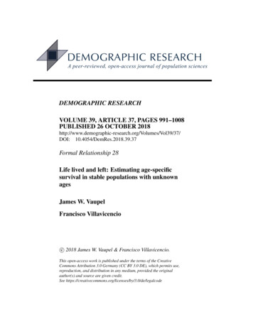
Demographic Research: Volume 39, Article 37time t a isea (t) e r Nea 1 (t).Na (t a) N(9*)Equation (9*) is an extension of our basic result (1*) to the case of observationsmade not continuously but at points in time t, t 1, t 2, etc., and is valid for anytime unit – minutes, hours, days, years, or decades. It is necessary, though, that the sameunit is used to measure time and age, and that the population is observed at regular timepoints. The Lexis diagram in Figure 2 provides some intuition about these concepts andrelationships.Figure 2:Lexis diagram illustrating the relationship between life lived andlife left in a discrete-time frameworkN(t) N0(t)N1(t)e rN2(t)e r3age / life livedN2 (t 1)N2(t 2)N1 (t)e r2N1(t 1)e r1N0(t)0t 1tt 1t 2timee0 (t), Ne1 (t), Ne2 (t), etc. followingNote: Life lived is captured by N (t), N0 (t), N1 (t 1), etc., and life left by NEquation (9*).An equivalent expression to the survival schedule in (2*) for the discrete case followsimmediately from (9*),(10*) a ea (t) e r Nea 1 (t)Na (t a)N ,e0 (t) e r Ne1 (t)N0 (t)Nhttp://www.demographic-research.org999

Vaupel & Villavicencio: Estimating age-specific survival in stable populations with unknown agesand the stable age structure defined in (6*) becomesNa (t)e ra Na (t a) N (t)N (t)ea 1 (t)ea (t) e r NN e ra.N (t)ca (11*)Figure 3 illustrates these two last results in a Lexis diagram: By following a stablepopulation with unknown ages from time t onward, and recording at each subsequente0 (t), Ne1 (t), Ne2 (t), etc.), we aretime step the number of remaining individuals alive (Nable to recover the cohort survival schedule a (left panel) and the stable age structure ca(right panel).Figure 3:Lexis diagrams illustrating the cohort survival schedule a (leftpanel) and the stable age structure ca (right panel) that can beestimated by following a stable population until extinctionNote: Stable population with unknown ages that is followed from time t onward, recording at each subsequent timestep the number of remaining individuals alive, and applying (10*) and (11*).4.2 Example of application with simulated dataTo check the validity of our results, we proceed with a reproducible example based onsimulating a stable population. Following the same idea that James Carey and colleaguesdeveloped in the study of survival patterns of captive medflies (Müller et al. 2004, 2007),1000http://www.demographic-research.org

Demographic Research: Volume 39, Article 37we observe a population at regular time points until its extinction, and we record theea (t) values at each time step. Applying (9*), (10*), and (11*), we use these values toNestimate the survival schedule used in the data simulation and the corresponding stableage structure. The R code (R Core Team 2018) to carry out this experiment is availablein the supplementary materials; only a few details are provided below.We adapt the same simplified example of a stable population used by Preston, Heuveline, and Guillot (2001: 138–141), so the reader can refer to that book to find additionalexplanation. Suppose there is a hypothetical population in which all individuals die before age 5, defined by the following life table:Table 1:Life table (survival schedule) used in the data simulationa012345 a1.000.600.400.200.050.00Function a gives the probability of surviving from age [0, 1) to age [a, a 1).All cohorts are driven by this survival schedule. We start with an initial population ofN0 (t 5) 105 individuals at age [0, 1) at time t 5. At time t 4, N1 (t 4) N0 (t 5) 1 individuals will reach age [1, 2), and N0 (t 4) N0 (t 5) er newly bornwill join the population, since r is the constant growth rate. Following the same procedurefor older ages and assuming a growth rate of r 0.01, at time t the population becomesstable with a population size of 234,248 individuals. The population counts by age aredisplayed in Table 2.Table 2:Population counts by age at time t of a simulated stable populationwith constant growth rate r 0.01aNa (t)0N0 (t 5) e5r 0 105 e0.05 1.00 105, 1271N0 (t 5) e4r 1 105 e0.04 0.60 62, 4492N0 (t 5) e3r 2 105 e0.03 0.40 41, 2183N0 (t 5) e2r 3 105 e0.02 0.20 20, 4044N0 (t 5) er 4 105 e0.01 0.05 5, 050 105 0.005N0 (t 5) 5TotalN (t) 234, 248 individuals 0From this population of 234,248 individuals we draw 100 random samples of 1,000individuals each. Then, ignoring the ages, we follow all of these samples until extinction,ea (t) values).recording at each time step the number of individuals who are still alive (Nhttp://www.demographic-research.org1001

Vaupel & Villavicencio: Estimating age-specific survival in stable populations with unknown agesAt each iteration, individuals randomly die depending on the corresponding age-specificprobabilities of death. Applying (9*), (10*), and (11*), we get estimates for the survivalschedule and the stable age structure for all samples. Finally, combining the results fromthe 100 samples, we obtain mean values and empirical confidence intervals for all theestimates and compare them with the survival schedule used in the data simulation andthe age structure of the whole population. The results displayed in Table 3 show that ourmethod to estimate a and ca for stable populations may provide serviceably accurateresults. Differences among the estimates and the true values observed at the populationlevel are due to the randomness in the data simulation and the sampling process, and alsobecause of the rounding to integer values of the population counts. All true values fallwithin the 95% empirical confidence intervals of the estimates.Estimates of the cohort survival schedule ba and the age structurecba of a simulated stable population, using information on life leftTable 3:a012345True values at thepopulation level aca ba (10*)cba (11*)1.000.600.400.200.050.001.000000.60131 [0.52142, 0.68716]0.40345 [0.33590, 0.46453]0.20128 [0.15901, 0.25306]0.04807 [0.03019, 0.07151]0.000000.44847 [0.42200, 0.47662]0.26636 [0.24147, 0.28867]0.17700 [0.15225, 0.19604]0.08738 [0.07130, 0.10583]0.02066 [0.01295, 0.00000Estimates from the samplesNote: Estimates from 100 samples of size 1,000 that are randomly taken from a stable population of 234,248 individuals. The samples are followed until death. Values between square brackets represent 95% empirical confidenceintervals.5. The 1805 cohort life table of Swedish femalesAs an example of application with actual data, we aim to recover the 1805 cohort lifetable of Swedish females by applying Equations (9*) and (10*) to data on populationcounts. The goal is to create a scenario in which we simulate the ‘capture’ of the Swedishfemales in 1805, ignoring their ages, and follow this group of individuals until extinction.First, we ‘capture’ the population in 1805, as in a census. Next, we follow thoseindividuals along the 19th century by recording the number of individuals still alive atea (t) values. Finally, applying (9*) weeach subsequent five-year period, obtaining the Nuse these estimates to compute the number of individuals in each age group at each timeperiod (Na (t a) values, see Figure 2), in order to apply (10*) and estimate the survival schedule a of the 1805 cohort of Swedish females (Figure 3, left panel). All the1002http://www.demographic-research.org

Demographic Research: Volume 39, Article 37data comes from the Human Mortality Database (2018) (henceforth HMD). The resultspresented below are fully reproducible from the R code (R Core Team 2018) and dataavailable in the supplementary materials.5.1 Estimation of the growth rateAn estimate of the stable growth rate r is needed to apply the formulas in this article. Thisparameter can be estimated in various ways because all scalable stable population parameters grow exponentially at the same rate, including the number of births and deaths, andpopulation size. Keyfitz and Caswell (2005, Chapter 5.2) provide an interesting discussion about how to estimate the growth rate from a single census, given the assumption of astable population in which all cohorts follow the same life table. However, their approachrequires knowledge of the number of individuals at a minimum of two different ages, andthe probability of surviving between them. This is not the case in a context in which theages of the population are unknown, and the survival schedule is estimated depending onthe growth rate r, as shown in (2*) and (10*).If the number of births B(t) at first observation can be assessed, one could simplyconsidere t)B(t) D(t)B(t) D(0,.r e (0, t)N (t)NWhen that information is not available, r can be estimated if the entire population (ora random sample) is observed at two time points t1 and t2 so that information is availableon N (t1 ) and N (t2 ). This may be the most convenient approach in many real-worldscenarios. If that is the case, ln N (t2 ) ln N (t1 )(12)r ,t2 t1a formula that follows from the definition of a stable population (Keyfitz and Caswell2005: 12). We use (12) to estimate the growth rate of the Swedish female population inthe 19th century, using the total populations counts of 1805 and 1895 from the HMD: ln 2,509,076 ln 1,249,946ln N (1895) ln N (1805) 0.00774.r 1895 18051895 18055.2 Reconstruction of the survival curveGiven the estimate of the population growth, we can proceed as in the example of Section 4.2, but with actual population counts from the HMD. First, we get the total pope0 (1805) 1,249,946. Next, we specify the numberulation in 1805, N (1805) Nhttp://www.demographic-research.org1003

Vaupel & Villavicencio: Estimating age-specific survival in stable populations with unknown agesof individuals from that initial population who are still alive in 1810. In terms of theavailable data, this corresponds to the number of Swedish females above age 5 in 1810,e5 (1805) 1,105,919. We follow the same procedure to obtainN5 (1810) Ne10 (1805) 1,007,581, N15 (1820) Ne15 (1805), and so on. AllN10 (1815) Nthese populatio

3.2 Life lived and left in stationary populations 995 3.3 The population of France from a life left perspective 997 4 Application 997 4.1 Life lived and left in a discrete-time framework 998 4.2 Example of application with simulated data 1000 5 The 1805 cohort life table of Swedish females 100