WIXLIB

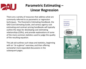
Parametric Estimating –Linear RegressionThere are a variety of resources that address what arecommonly referred to as parametric or regressiontechniques. The Parametric Estimating Handbook, theGAO Cost Estimating Guide, and various agency costestimating and contract pricing handbooks will typicallyoutline the steps for developing cost estimatingrelationships (CERs), and provide explanations of someof the more common statistics used to judge the qualityof the resulting equation.This job aid outlines such steps and statistics, beginningwith an “at-a-glance” overview, and then offeringsomewhat more expanded discussions in thesubsequent pages.

Developing Cost Estimating Relationships

Developing Cost Estimating Relationships

Developing Cost Estimating Relationships

Developing Cost Estimating RelationshipsThe term “cost estimating relationship” or CER isused here in the context of an equation where wepredict the outcome of one variable as a function ofthe behavior of one or more other variables.We refer to the predicted variable as the dependentor Y variable. Those variables that can be said toexplain or drive the behavior of the predictedvariable are consequently called explanatoryvariables or cost drivers, also known as theindependent or X variables.The terms CERs, equations, or models are oftenused interchangeably, although the term “model” issometimes reserved to describe an assemblage ofCERs, equations, or factors such as is often the casewith respect to a software cost estimating “model”.

Identification of Cost DriversIs it possible for a variable to be a major cost driver,but not be a significant cost driver?Consider the engine in a car. The engine is both amajor cost element of the car’s price, and a majorcost driver in that variations in the size of the enginegenerally have a significant impact on the cost.However, if you were trying to discern why the pricesof a certain set of cars varied, and those cars all hadengines of a similar size, then the engine size wouldnot be “significant” in that the engine size would notdiscriminate between, or explain, differences in theprices.Nevertheless, it would still be important to documentthe engine size as being a major cost driver in theevent you were faced with estimating the price of acar with a different engine size. In that case, theengine size might then become a significant costdriver.

Specification of the RelationshipGenerally speaking, there are two approaches tofitting data. In one approach you simply rely on thedata to “speak for itself”. The analyst eitherobserves patterns in the data and makes aselection, or they run successive regressions ofvarying types and determine which equation “bestfits” the data. This approach is best suited forsituations where there is an abundance of data, orcompelling patterns in the data.However, the analyst faced with smaller data setsand less compelling data is better advised to firstseek the expectations of the subject matter experts,hypothesize a relationship, and then test thathypothesis. This makes for a more sound anddefensible estimating relationship.

Data CollectionOne challenge that analysts sometimes face is ashortage of similar items for comparison. Whensearching for “similar” items, the analyst shouldconsider the level at which that similarity needexist. For example, an analyst pricing a componenton a stealth ship need not unnecessarily constrainthemselves to stealth ships when it is possible thatthe same or similar component is used on a varietyof ships, and perhaps ground vehicles and aircraft aswell.Another consideration for expanding the number ofsimilar items is to estimate at lower levels of thework breakdown structure when necessary, andwhen such data exists.Familiarize yourself with the data bases that yourorganization and others maintain.

Normalizing the DataYou probably learned at some point in a scienceclass that when constructing experiments to studythe effects of one thing upon another that it wasimportant to hold everything else constant as muchas possible. That’s essentially the idea behindnormalizing the data, to get a more true measure ofthe relationship between the Y and X variables.One of the other benefits of going through theprocess of making these adjustments in the data isthat it forces us to develop a better understandingof the effects that each of these factors has on“cost”, such as the changes in quantity, technology,material, labor differences, etc.Look for checklists that your agency and others usewhen comparing prices, costs, hours, etc.

Graphical/Visual Analysis of the DataIf you’re counting on the R2, T statistic, F statistic,standard error, or coefficient of variation to tell youthat you are not properly fitting the data, or thatyou have outliers or gaps in the data, then get readyto be disappointed, because they won’t!Histograms, number lines, scatterplots, and more.There is just no substitution for looking at the data.Hopefully the scatterplots will be consistent withyour expectations from the specification step. Ifnot, then this is the opportunity to reengage withyour subject matter experts.Scatterplots may highlight subgroups or classeswithin the data; changes in the cost estimatingrelationship over the range of the data; andunusual values within the data set.

Selecting a Fitting Approach for the DataThis step is the extension of the specification andvisual analysis steps. We will concern ourselveshere with linear relationships. See the Nonlinearjob aid for discussions on fitting nonlinear data.The most common linear relationship is a factor.The use of a factor presumes a direct proportionalrelationship between the X and Y variables.A factor can be derived from a single data point orfrom a set of data points. Regression can be used toderive a factor when dealing with a set of datapoints by specifying a zero intercept or “constant iszero” in applications such as Excel. (See the Factorsjob aid for further discussion on the use of factors.)

The Linear EquationThe equation of a line has been represented by ahost of different letters and characters, at ourearliest ages commonly by (y mx b).One of the assumptions regarding the regressionline is that there is a distribution of Y values aroundevery point on the line. When we fit a line throughthe data, the resulting line represents the mean oraverage value of Y for every value of X.So we need to recognize there is arange of possible Y values for agiven value of X, and that theestimated Y value is essentially theaverage of the possible outcomes.For example, given the equation:TV Price 76.00 13.25 (Inches) 76.00 13.25 (32) 500We would say that the average price for a TV with adiagonal of 32 inches is estimated to be 500.

Determining the Confidence LevelThe T-test is a hypothesis test. The null hypothesis isthat there is no relationship between the X and Yvariables, in which case the slope would equal zero.The alternate hypothesis is that the X and Y variablesare related, which would be evidenced by a positiveor negative slope.The test requires that we measure how far the slopeis from zero in units of standard deviations (T calc) sothat we can associate the distance with a measure ofprobability. Most regression applications report theT calc value and the probability associated with it.The probability can either be stated in terms of thelevel of significance or as the level of confidence.Some applications report “P” or a “P value” which isthe level of significance. A “P value” of 0.10 equatesto a 0.90 or 90% level of confidence. Exercising somelatitude with the terminology, we might say that weare 90% confident that the X and Y variables arerelated.The analyst then needs to decide what constitutes anacceptable level of confidence that would warrantconsidering the equation.

The ANOVA TableThe next two topics will makereference to SSE, SSR, and SST.They also refer to the Degreesof Freedom (DF) notation:n–por alternativelyn–k–1DF is the adjustment made tosample statistics to betterestimate the associatedpopulation parameters (e.g. thesample variance as an estimateof the population variance).In the diagram, Yi is the actualvalue of Y for a given X.The Y with the hat or symbolis the predicted value of Y for agiven X.The Y with the line over it(pronounced Y bar) representsthe average of all the Y values.

How Accurate is theEquation?Ideally we would test the accuracy of the equationby reserving some of the data points, and thenassessing how well we estimated those points basedon the equation resulting from the remaining data.Unfortunately, due to the far too common problemof small data sets we cannot afford the luxury ofreserving data points. As an alternative, we measurehow well we fit the data used to create the equation.The SSE is the sum of the squared errors around theregression line. By dividing the SSE by “n – p” oralternatively by “n – k – 1”, we arrive at the varianceof the equation, and what we might loosely call theaverage squared estimating error.The square root of the variance is commonly calledthe standard error or standard error of the estimate.Again, we could loosely interpret this as the averageestimating error.By comparing the standard error to the averagevalue of Y we get a relative measure of variabilitycalled the coefficient of variation, which we mightthink of as an average percent estimating error.

How much of thevariation in Y has beenexplained?Presumably we are developing a CER to explain thevariation in our Y variable for the purpose of betterestimating it. It seems reasonable then to ask howmuch of the variation in the Y variable that we havebeen able to account for.The sum of squares total, or SST, represents the totalsquared variation around the mean of Y. The sum ofsquares regression, or SSR, represents the portion ofthe variation in the SST that we have accounted forin the equation. You might say SSR is the variation inY that we can associate with the variation in X.R squared is the ratio of the explained variation (SSR)to the total variation (SST). While calculated as adecimal value between 0 and 1, it’s commonlyexpressed as a percentage between 0 and 100. If theequation bisected all of the data points, R squaredwould be 100%, meaning all of the variation in Ywould have been explained by the variation in X.R squared should not be used to imply causality, butrather used to support the causality suppositionfrom the step where we identified what we believedto be causal cost drivers.

X and Y OutliersWe want to be aware of unusual values in the data for a number of reasons. It mayindicate deficiencies in how we’ve normalized the data. It could be that there aredifferences in the data that either we were unaware of, or if we were aware of, we didn’tknow the impact those differences would have. And there is the concern of how thatunusual value impacts our ability to fit the remaining data.One test for what we call outliers, is to measure how far an X or Y value is from the meanof X or Y, in units of standard deviations. A more robust technique for the X variable is tocalculate the leverage value for each X. Well-named, the higher the leverage value, themore leverage a particular X data point has on the slope and intercept of the equation.Outliers should be investigated prior to consideration for removal from the data set.When does an X or Y become anoutlier? It’s subjective, but oneconvention is that when a value ismore than plus or minus twostandard deviations from themean it is considered an outlier.Leverage uses P (the number ofcoefficients in the equation)divided by “n” (the sample size).A multiplier of 2 or 3 times P/n isused as the point at which an Xobservation becomes an outlier.