Transcription
LECTURE NOTESCourse 6.041-6.431M.I.T.FALL 2000Introduction to ProbabilityDimitri P. Bertsekas and John N. TsitsiklisProfessors of Electrical Engineering and Computer ScienceMassachusetts Institute of TechnologyCambridge, MassachusettsThese notes are copyright-protected but may be freely distributed forinstructional nonprofit pruposes.
Contents1. Sample Space and Probability1.1.1.2.1.3.1.4.1.5.1.6.1.7.Sets . . . . . . . . . .Probabilistic Models . . .Conditional Probability .Independence . . . . . .Total Probability TheoremCounting . . . . . . .Summary and Discussion2. Discrete Random Variables2.1.2.2.2.3.2.4.2.5.2.6.2.7.2.8. . . . .and. . . . . . . . . . .Bayes’. . . . . . . . . . . . .Rule. . . . . . . . . . . . . . . . . . . . .Basic Concepts . . . . . . . . . . . .Probability Mass Functions . . . . . .Functions of Random Variables . . . . .Expectation, Mean, and Variance . . . .Joint PMFs of Multiple Random VariablesConditioning . . . . . . . . . . . . .Independence . . . . . . . . . . . . .Summary and Discussion . . . . . . .3. General Random Variables3.1.3.2.3.3.3.4.3.5.3.6.3.7. . . . . . . . . . . . . . . . . . . . . . . . . . . . . . . .Continuous Random Variables and PDFsCumulative Distribution Functions . . .Normal Random Variables . . . . . . .Conditioning on an Event . . . . . . .Multiple Continuous Random Variables .Derived Distributions . . . . . . . . .Summary and Discussion . . . . . . .4. Further Topics on Random Variables and Expectations . . . . . .4.1. Transforms . . . . . . . . . . . . . . . . . . . . . . . . . . .4.2. Sums of Independent Random Variables - Convolutions . . . . . . .iii
iv4.3.4.4.4.5.4.6.4.7.ContentsConditional Expectation as a Random Variable . .Sum of a Random Number of Independent RandomCovariance and Correlation . . . . . . . . . .Least Squares Estimation . . . . . . . . . . .The Bivariate Normal Distribution . . . . . . . . . .Variables. . . . . . . . . . . . . .5. The Bernoulli and Poisson Processes . . . . . . . . . . . . . .5.1. The Bernoulli Process . . . . . . . . . . . . . . . . . . . . . .5.2. The Poisson Process . . . . . . . . . . . . . . . . . . . . . . .6. Markov Chains . . . . . . . . . . . . . . . . . . . . . . .6.1.6.2.6.3.6.4.6.5.Discrete-Time Markov Chains . . . . . .Classification of States . . . . . . . . . .Steady-State Behavior . . . . . . . . . .Absorption Probabilities and Expected TimeMore General Markov Chains . . . . . . .to. . . . . . . . . . . . . . . .Absorption. . . . . .7. Limit Theorems . . . . . . . . . . . . . . . . . . . . . . .7.1.7.2.7.3.7.4.7.5.Some Useful Inequalities . . . . .The Weak Law of Large Numbers .Convergence in Probability . . . .The Central Limit Theorem . . .The Strong Law of Large Numbers.
PrefaceThese class notes are the currently used textbook for “Probabilistic SystemsAnalysis,” an introductory probability course at the Massachusetts Institute ofTechnology. The text of the notes is quite polished and complete, but the problems are less so.The course is attended by a large number of undergraduate and graduatestudents with diverse backgrounds. Acccordingly, we have tried to strike a balance between simplicity in exposition and sophistication in analytical reasoning.Some of the more mathematically rigorous analysis has been just sketched orintuitively explained in the text, so that complex proofs do not stand in the wayof an otherwise simple exposition. At the same time, some of this analysis andthe necessary mathematical results are developed (at the level of advanced calculus) in theoretical problems, which are included at the end of the correspondingchapter. The theoretical problems (marked by *) constitute an important component of the text, and ensure that the mathematically oriented reader will findhere a smooth development without major gaps.We give solutions to all the problems, aiming to enhance the utility ofthe notes for self-study. We have additional problems, suitable for homeworkassignment (with solutions), which we make available to instructors.Our intent is to gradually improve and eventually publish the notes as atextbook, and your comments will be appreciatedDimitri P. Bertsekasbertsekas@lids.mit.eduJohn N. Tsitsiklisjnt@mit.eduv
1Sample Space Sets . . . . . . . . . .Probabilistic Models . . .Conditional Probability .Total Probability TheoremIndependence . . . . . .Counting . . . . . . .Summary and Discussion. . . .and. . . . . . . . . .Bayes’. . . . . . . . . . . . .Rule. . . . . . . p. 3. p. 6p. 16p. 25p. 31p. 41p. 481
2Sample Space and ProbabilityChap. 1“Probability” is a very useful concept, but can be interpreted in a number ofways. As an illustration, consider the following.A patient is admitted to the hospital and a potentially life-saving drug isadministered. The following dialog takes place between the nurse and aconcerned relative.RELATIVE: Nurse, what is the probability that the drug will work?NURSE: I hope it works, we’ll know tomorrow.RELATIVE: Yes, but what is the probability that it will?NURSE: Each case is different, we have to wait.RELATIVE: But let’s see, out of a hundred patients that are treated undersimilar conditions, how many times would you expect it to work?NURSE (somewhat annoyed): I told you, every person is different, for someit works, for some it doesn’t.RELATIVE (insisting): Then tell me, if you had to bet whether it will workor not, which side of the bet would you take?NURSE (cheering up for a moment): I’d bet it will work.RELATIVE (somewhat relieved): OK, now, would you be willing to losetwo dollars if it doesn’t work, and gain one dollar if it does?NURSE (exasperated): What a sick thought! You are wasting my time!In this conversation, the relative attempts to use the concept of probability todiscuss an uncertain situation. The nurse’s initial response indicates that themeaning of “probability” is not uniformly shared or understood, and the relativetries to make it more concrete. The first approach is to define probability interms of frequency of occurrence, as a percentage of successes in a moderatelylarge number of similar situations. Such an interpretation is often natural. Forexample, when we say that a perfectly manufactured coin lands on heads “withprobability 50%,” we typically mean “roughly half of the time.” But the nursemay not be entirely wrong in refusing to discuss in such terms. What if thiswas an experimental drug that was administered for the very first time in thishospital or in the nurse’s experience?While there are many situations involving uncertainty in which the frequency interpretation is appropriate, there are other situations in which it isnot. Consider, for example, a scholar who asserts that the Iliad and the Odysseywere composed by the same person, with probability 90%. Such an assertionconveys some information, but not in terms of frequencies, since the subject isa one-time event. Rather, it is an expression of the scholar’s subjective belief. One might think that subjective beliefs are not interesting, at least from amathematical or scientific point of view. On the other hand, people often haveto make choices in the presence of uncertainty, and a systematic way of makinguse of their beliefs is a prerequisite for successful, or at least consistent, decision
Sec. 1.1Sets3making.In fact, the choices and actions of a rational person, can reveal a lot aboutthe inner-held subjective probabilities, even if the person does not make conscioususe of probabilistic reasoning. Indeed, the last part of the earlier dialog was anattempt to infer the nurse’s beliefs in an indirect manner. Since the nurse waswilling to accept a one-for-one bet that the drug would work, we may inferthat the probability of success was judged to be at least 50%. And had thenurse accepted the last proposed bet (two-for-one), that would have indicated asuccess probability of at least 2/3.Rather than dwelling further into philosophical issues about the appropriateness of probabilistic reasoning, we will simply take it as a given that the theoryof probability is useful in a broad variety of contexts, including some where theassumed probabilities only reflect subjective beliefs. There is a large body ofsuccessful applications in science, engineering, medicine, management, etc., andon the basis of this empirical evidence, probability theory is an extremely usefultool.Our main objective in this book is to develop the art of describing uncertainty in terms of probabilistic models, as well as the skill of probabilisticreasoning. The first step, which is the subject of this chapter, is to describethe generic structure of such models, and their basic properties. The models weconsider assign probabilities to collections (sets) of possible outcomes. For thisreason, we must begin with a short review of set theory.1.1 SETSProbability makes extensive use of set operations, so let us introduce at theoutset the relevant notation and terminology.A set is a collection of objects, which are the elements of the set. If S isa set and x is an element of S, we write x S. If x is not an element of S, wewrite x / S. A set can have no elements, in which case it is called the emptyset, denoted by Ø.Sets can be specified in a variety of ways. If S contains a finite number ofelements, say x1 , x2 , . . . , xn , we write it as a list of the elements, in braces:S {x1 , x2 , . . . , xn }.For example, the set of possible outcomes of a die roll is {1, 2, 3, 4, 5, 6}, and theset of possible outcomes of a coin toss is {H, T }, where H stands for “heads”and T stands for “tails.”If S contains infinitely many elements x1 , x2 , . . ., which can be enumeratedin a list (so that there are as many elements as there are positive integers) wewriteS {x1 , x2 , . . .},
4Sample Space and ProbabilityChap. 1and we say that S is countably infinite. For example, the set of even integerscan be written as {0, 2, 2, 4, 4, . . .}, and is countably infinite.Alternatively, we can consider the set of all x that have a certain propertyP , and denote it by{x x satisfies P }.(The symbol “ ” is to be read as “such that.”) For example the set of evenintegers can be written as {k k/2 is integer}. Similarly, the set of all scalars xin the interval [0, 1] can be written as {x 0 x 1}. Note that the elements xof the latter set take a continuous range of values, and cannot be written downin a list (a proof is sketched in the theoretical problems); such a set is said to beuncountable.If every element of a set S is also an element of a set T , we say that Sis a subset of T , and we write S T or T S. If S T and T S, thetwo sets are equal, and we write S T . It is also expedient to introduce auniversal set, denoted by Ω, which contains all objects that could conceivablybe of interest in a particular context. Having specified the context in terms of auniversal set Ω, we only consider sets S that are subsets of Ω.Set OperationsThe complement of a set S, with respect to the universe Ω, is the set {x Ω x / S} of all elements of Ω that do not belong to S, and is denoted by S c .Note that Ωc Ø.The union of two sets S and T is the set of all elements that belong to Sor T (or both), and is denoted by S T . The intersection of two sets S and Tis the set of all elements that belong to both S and T , and is denoted by S T .Thus,S T {x x S or x T },S T {x x S and x T }.In some cases, we will have to consider the union or the intersection of several,even infinitely many sets, defined in the obvious way. For example, if for everypositive integer n, we are given a set Sn , then Sn S1 S2 · · · {x x Sn for some n},n 1and Sn S1 S2 · · · {x x Sn for all n}.n 1Two sets are said to be disjoint if their intersection is empty. More generally,several sets are said to be disjoint if no two of them have a common element. Acollection of sets is said to be a partition of a set S if the sets in the collectionare disjoint and their union is S.
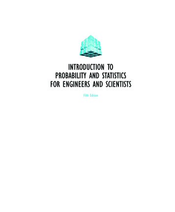
Sec. 1.1Sets5If x and y are two objects, we use (x, y) to denote the ordered pair of xand y. The set of scalars (real numbers) is denoted by ; the set of pairs (ortriplets) of scalars, i.e., the two-dimensional plane (or three-dimensional space,respectively) is denoted by 2 (or 3 , respectively).Sets and the associated operations are easy to visualize in terms of Venndiagrams, as illustrated in Fig. )(f)Figure 1.1: Examples of Venn diagrams. (a) The shaded region is S T . (b)The shaded region is S T . (c) The shaded region is S T c . (d) Here, T S.The shaded region is the complement of S. (e) The sets S, T , and U are disjoint.(f) The sets S, T , and U form a partition of the set Ω.The Algebra of SetsSet operations have several properties, which are elementary consequences of thedefinitions. Some examples are:S TS (T U )(S c )cS Ω T S, (S T ) (S U ), S, Ω,S (T U )S (T U )S ScS Ω (S T ) U, (S T ) (S U ), Ø, S.Two particularly useful properties are given by de Morgan’s laws whichstate that c c Sn Snc ,Sn Snc .nnnnTo establish the first law, suppose that x ( n SnThen, x / n Sn , whichimplies that for every n, we have x / Sn . Thus, x belongs to the complement)c .
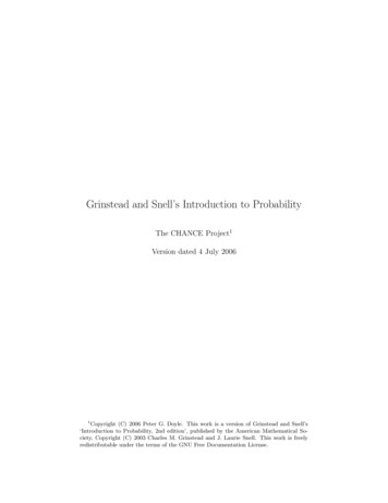
6Sample Space and ProbabilityChap. 1of every Sn , and xn n Snc . This shows that ( n Sn )c n Snc . The converseinclusion is established by reversing the above argument, and the first law follows.The argument for the second law is similar.1.2 PROBABILISTIC MODELSA probabilistic model is a mathematical description of an uncertain situation.It must be in accordance with a fundamental framework that we discuss in thissection. Its two main ingredients are listed below and are visualized in Fig. 1.2.Elements of a Probabilistic Model The sample space Ω, which is the set of all possible outcomes of anexperiment. The probability law, which assigns to a set A of possible outcomes(also called an event) a nonnegative number P(A) (called the probability of A) that encodes our knowledge or belief about the collective“likelihood” of the elements of A. The probability law must satisfycertain properties to be introduced shortly.ProbabilityLawEvent BExperimentEvent ASample Space Ω(Set of Outcomes)P(B)P(A)ABEventsFigure 1.2: The main ingredients of a probabilistic model.Sample Spaces and EventsEvery probabilistic model involves an underlying process, called the experiment, that will produce exactly one out of several possible outcomes. The setof all possible outcomes is called the sample space of the experiment, and isdenoted by Ω. A subset of the sample space, that is, a collection of possible
Sec. 1.2Probabilistic Models7outcomes, is called an event.† There is no restriction on what constitutes anexperiment. For example, it could be a single toss of a coin, or three tosses,or an infinite sequence of tosses. However, it is important to note that in ourformulation of a probabilistic model, there is only one experiment. So, threetosses of a coin constitute a single experiment, rather than three experiments.The sample space of an experiment may consist of a finite or an infinitenumber of possible outcomes. Finite sample spaces are conceptually and mathematically simpler. Still, sample spaces with an infinite number of elements arequite common. For an example, consider throwing a dart on a square target andviewing the point of impact as the outcome.Choosing an Appropriate Sample SpaceRegardless of their number, different elements of the sample space should bedistinct and mutually exclusive so that when the experiment is carried out,there is a unique outcome. For example, the sample space associated with theroll of a die cannot contain “1 or 3” as a possible outcome and also “1 or 4” asanother possible outcome. When the roll is a 1, the outcome of the experimentwould not be unique.A given physical situation may be modeled in several different ways, depending on the kind of questions that we are interested in. Generally, the samplespace chosen for a probabilistic model must be collectively exhaustive, in thesense that no matter what happens in the experiment, we always obtain an outcome that has been included in the sample space. In addition, the sample spaceshould have enough detail to distinguish between all outcomes of interest to themodeler, while avoiding irrelevant details.Example 1.1. Consider two alternative games, both involving ten successive cointosses:Game 1: We receive 1 each time a head comes up.Game 2: We receive 1 for every coin toss, up to and including the first timea head comes up. Then, we receive 2 for every coin toss, up to the secondtime a head comes up. More generally, the dollar amount per toss is doubledeach time a head comes up.† Any collection of possible outcomes, including the entire sample space Ω andits complement, the empty set Ø, may qualify as an event. Strictly speaking, however,some sets have to be excluded. In particular, when dealing with probabilistic modelsinvolving an uncountably infinite sample space, there are certain unusual subsets forwhich one cannot associate meaningful probabilities. This is an intricate technical issue,involving the mathematics of measure theory. Fortunately, such pathological subsetsdo not arise in the problems considered in this text or in practice, and the issue can besafely ignored.
8Sample Space and ProbabilityChap. 1In game 1, it is only the total number of heads in the ten-toss sequence that matters, while in game 2, the order of heads and tails is also important. Thus, ina probabilistic model for game 1, we can work with a sample space consisting ofeleven possible outcomes, namely, 0, 1, . . . , 10. In game 2, a finer grain descriptionof the experiment is called for, and it is more appropriate to let the sample spaceconsist of every possible ten-long sequence of heads and tails.Sequential ModelsMany experiments have an inherently sequential character, such as for exampletossing a coin three times, or observing the value of a stock on five successivedays, or receiving eight successive digits at a communication receiver. It is thenoften useful to describe the experiment and the associated sample space by meansof a tree-based sequential description, as in Fig. 1.3.Sample SpacePair of RollsSequential TreeDescription4132nd Roll1, 11, 21, 31, 42RootLeaves2311231st Roll44Figure 1.3: Two equivalent descriptions of the sample space of an experimentinvolving two rolls of a 4-sided die. The possible outcomes are all the ordered pairsof the form (i, j), where i is the result of the first roll, and j is the result of thesecond. These outcomes can be arranged in a 2-dimensional grid as in the figureon the left, or they can be described by the tree on the right, which reflects thesequential character of the experiment. Here, each possible outcome correspondsto a leaf of the tree and is associated with the unique path from the root to thatleaf. The shaded area on the left is the event {(1, 4), (2, 4), (3, 4), (4, 4)} that theresult of the second roll is 4. That same event can be described as a set of leaves,as shown on the right. Note also that every node of the tree can be identified withan event, namely, the set of all leaves downstream from that node. For example,the node labeled by a 1 can be identified with the event {(1, 1), (1, 2), (1, 3), (1, 4)}that the result of the first roll is 1.Probability LawsSuppose we have settled on the sample space Ω associated with an experiment.
Sec. 1.2Probabilistic Models9Then, to complete the probabilistic model, we must introduce a probabilitylaw. Intuitively, this specifies the “likelihood” of any outcome, or of any set ofpossible outcomes (an event, as we have called it earlier). More precisely, theprobability law assigns to every event A, a number P(A), called the probabilityof A, satisfying the following axioms.Probability Axioms1. (Nonnegativity) P(A) 0, for every event A.2. (Additivity) If A and B are two disjoint events, then the probabilityof their union satisfiesP(A B) P(A) P(B).Furthermore, if the sample space has an infinite number of elementsand A1 , A2 , . . . is a sequence of disjoint events, then the probability oftheir union satisfiesP(A1 A2 · · ·) P(A1 ) P(A2 ) · · ·3. (Normalization) The probability of the entire sample space Ω isequal to 1, that is, P(Ω) 1.In order to visualize a probability law, consider a unit of mass which isto be “spread” over the sample space. Then, P(A) is simply the total massthat was assigned collectively to the elements of A. In terms of this analogy, theadditivity axiom becomes quite intuitive: the total mass in a sequence of disjointevents is the sum of their individual masses.A more concrete interpretation of probabilities is in terms of relative frequencies: a statement such as P(A) 2/3 often represents a belief that event Awill materialize in about two thirds out of a large number of repetitions of theexperiment. Such an interpretation, though not always appropriate, can sometimes facilitate our intuitive understanding. It will be revisited in Chapter 7, inour study of limit theorems.There are many natural properties of a probability law which have not beenincluded in the above axioms for the simple reason that they can be derivedfrom them. For example, note that the normalization and additivity axiomsimply that1 P(Ω) P(Ω Ø) P(Ω) P(Ø) 1 P(Ø),and this shows that the probability of the empty event is 0:P(Ø) 0.
10Sample Space and ProbabilityChap. 1As another example, consider three disjoint events A1 , A2 , and A3 . We can usethe additivity axiom for two disjoint events repeatedly, to obtain P(A1 A2 A3 ) P A1 (A2 A2 ) P(A1 ) P(A2 A3 ) P(A1 ) P(A2 ) P(A3 ).Proceeding similarly, we obtain that the probability of the union of finitely manydisjoint events is always equal to the sum of the probabilities of these events.More such properties will be considered shortly.Discrete ModelsHere is an illustration of how to construct a probability law starting from somecommon sense assumptions about a model.Example 1.2. Coin tosses.Consider an experiment involving a single cointoss. There are two possible outcomes, heads (H) and tails (T ). The sample spaceis Ω {H, T }, and the events are{H, T }, {H}, {T }, Ø.If the coin is fair, i.e., if we believe that heads and tails are “equally likely,” weshould assign equal probabilities to the two possible outcomes and specify thatP {H} P {T } 0.5. The additivity axiom implies that P {H, T } P {H} P {T } 1,which is consistent with the normalization axiom. Thus, the probability law is givenby P {H, T } 1, P {H} 0.5, P {T } 0.5,P(Ø) 0,and satisfies all three axioms.Consider another experiment involving three coin tosses. The outcome willnow be a 3-long string of heads or tails. The sample space isΩ {HHH, HHT, HT H, HT T, T HH, T HT, T T H, T T T }.We assume that each possible outcome has the same probability of 1/8. Let usconstruct a probability law that satisfies the three axioms. Consider, as an example,the eventA {exactly 2 heads occur} {HHT, HT H, T HH}.
Sec. 1.2Probabilistic Models11Using additivity, the probability of A is the sum of the probabilities of its elements: P {HHT, HT H, T HH} P {HHT } P {HT H} P {T HH}111 8883 .8 Similarly, the probability of any event is equal to 1/8 times the number of possibleoutcomes contained in the event. This defines a probability law that satisfies thethree axioms.By using the additivity axiom and by generalizing the reasoning in thepreceding example, we reach the following conclusion.Discrete Probability LawIf the sample space consists of a finite number of possible outcomes, then theprobability law is specified by the probabilities of the events that consist ofa single element. In particular, the probability of any event {s1 , s2 , . . . , sn }is the sum of the probabilities of its elements: P {s1 , s2 , . . . , sn } P {s1 } P {s2 } · · · P {sn } . In the special case where the probabilities P {s1 }), . . . , P({sn } are all thesame (by necessity equal to 1/n, in view of the normalization axiom), we obtainthe following.Discrete Uniform Probability LawIf the sample space consists of n possible outcomes which are equally likely(i.e., all single-element events have the same probability), then the probability of any event A is given byP(A) Number of elements of A.nLet us provide a few more examples of sample spaces and probability laws.Example 1.3. Dice. Consider the experiment of rolling a pair of 4-sided dice (cf.Fig. 1.4). We assume the dice are fair, and we interpret this assumption to mean
12Sample Space and ProbabilityChap. 1that each of the sixteen possible outcomes [ordered pairs (i, j), with i, j 1, 2, 3, 4],has the same probability of 1/16. To calculate the probability of an event, wemust count the number of elements of event and divide by 16 (the total number ofpossible outcomes). Here are some event probabilities calculated in this way: P {the sum of the rolls is even} 8/16 1/2,P {the sum of the rolls is odd} 8/16 1/2, P {the first roll is equal to the second} 4/16 1/4, P {the first roll is larger than the second} 6/16 3/8, P {at least one roll is equal to 4} 7/16.Sample SpacePair of Rolls432nd RollEvent{at least one roll is a 4}Probability 7/16211231st Roll4Event{the first roll is equal to the second}Probability 4/16Figure 1.4: Various events in the experiment of rolling a pair of 4-sided dice,and their probabilities, calculated according to the discrete uniform law.Continuous ModelsProbabilistic models with continuous sample spaces differ from their discretecounterparts in that the probabilities of the single-element events may not besufficient to characterize the probability law. This is illustrated in the followingexamples, which also illustrate how to generalize the uniform probability law tothe case of a continuous sample space.
Sec. 1.2Probabilistic Models13Example 1.4. A wheel of fortune is continuously calibrated from 0 to 1, so thepossible outcomes of an experiment consisting of a single spin are the numbers inthe interval Ω [0, 1]. Assuming a fair wheel, it is appropriate to consider alloutcomes equally likely, but what is the probability of the event consisting of asingle element? It cannot be positive, because then, using the additivity axiom, itwould follow that events with a sufficiently large number of elements would haveprobability larger than 1. Therefore, the probability of any event that consists of asingle element must be 0.In this example, it makes sense to assign probability b a to any subinterval[a, b] of [0, 1], and to calculate the probability of a more complicated set by evaluating its “length.”† This assignment satisfies the three probability axioms andqualifies as a legitimate probability law.Example 1.5. Romeo and Juliet have a date at a given time, and each will arriveat the meeting place with a delay between 0 and 1 hour, with all pairs of delaysbeing equally likely. The first to arrive will wait for 15 minutes and will leave if theother has not yet arrived. What is the probability that they will meet?Let us use as sample space the square Ω [0, 1] [0, 1], whose elements arethe possible pairs of delays for the two of them. Our interpretation of “equallylikely” pairs of delays is to let the probability of a subset of Ω be equal to its area.This probability law satisfies the three probability axioms. The event that Romeoand Juliet will meet is the shaded region in Fig. 1.5, and its probability is calculatedto be 7/16.Properties of Probability LawsProbability laws have a number of properties, which can be deduced from theaxioms. Some of them are summarized below.Some Properties of Probability LawsConsider a probability law, and let A, B, and C be events.(a) If A B, then P(A) P(B).(b) P(A B) P(A) P(B) P(A B).(c) P(A B) P(A) P(B).(d) P(A B C) P(A) P(Ac B) P(Ac B c C).† The “length” of a subset S of [0, 1] is the integral dt, which is defined, forS“nice” sets S, in the usual calculus sense. For unusual sets, this integral may not bewell defined mathematically, but such issues belong to a more advanced treatment ofthe subject.
14Sample Space and ProbabilityChap. 1y1M1/401/41xFigure 1.5: The event M that Romeo and Juliet will arrive within 15 minutesof each other (cf. Example 1.5) isM (x, y) x y 1/4, 0 x 1, 0 y 1 ,and is shaded in the figure. The area of M is 1 minus the area of the two unshadedtriangles, or 1 (3/4) · (3/4) 7/16. Thus, the probability of meeting is 7/16.These properties, and other similar ones, can be visualized and verifiedgraphically using Venn diagrams, as in Fig. 1.6. For a further example, notethat we can apply property (c) repeatedly and obtain the inequalitynP(A1 A2 · · · An ) P(Ai ).i 1In more detail, let us apply property (c) to the sets A1 and A2 · · · An , toobtainP(A1 A2 · · · An ) P(A1 ) P(A2 · · · An ).We also apply property (c) to the sets A2 and A3 · · · An to obtainP(A2 · · · An ) P(A2 ) P(A3 · · · An ),continue similarly, and finally add.Models and RealityUsing the framework of probability theory to analyze a physical but uncertainsituation, involves two distinct stages.(a) In the first stage, we construct a probabilistic model,
Introduction to Probability Dimitri P. Bertsekas and John N. Tsitsiklis Professors of Electrical Engineering and Computer Science Massachusetts Institute of Technology Cambridge, Massachusetts These notes are copyright-protected but may be freely distributed for instructional nonprofit pruposes.