Transcription
CELLULAR MOBILECOMMUNICATION1
UNIT IINTRODUCTION TO WIRELESS MOBILECOMMUNICATION2
Introduction: In 1897, Guglielmo Marconi first demonstrated radio’s ability to providecontinuous contact with ships sailing the English channel. During the past 10 years, fueled by Digital and RF circuit fabrication improvements New VLSI technologies Other miniaturization technologies(e.g., passive components) The mobile communications industry has grown by orders of magnitude. The trends will continue at an even greater pace during the next decade.3
Evolution of Mobile Radio Communications4
In 1934, AM mobile communication systems for municipal police radio systems. Vehicle ignition noise was a major problem. In 1946, FM mobile communications for the first public mobile telephone service Each system used a single, high-powered transmitter and large tower to coverdistances of over 50 km. Used 120 kHz of RF bandwidth in a half-duplex mode. (push-to-talk release-tolisten systems.) Large RF bandwidth was largely due to the technology difficulty (in massproducing tight RF filter and low-noise, front-end receiver amplifiers.) In 1950, the channel bandwidth was cut in half to 60kHZ due to improvedtechnology. By the mid 1960s, the channel bandwidth again was cut to 30 kHZ. Thus, from WWII to the mid 1960s, the spectrum efficiency was improved only afactor of 4 due to the technology advancements.5
Also in 1950s and 1960s, automatic channel truncking was introducedin IMTS(Improved Mobile Telephone Service.) offering full duplex, auto-dial, auto-trunking became saturated quickly By 1976, has only twelve channels and could only serve 543customers in New York City of 10 millions populations. Cellular radiotelephone Developed in 1960s by Bell Lab and others The basic idea is to reuse the channel frequency at a sufficient distance toincrease the spectrum efficiency. But the technology was not available to implement until the late 1970s.(mainly the microprocessor and DSP technologies.)6
In 1983, AMPS (Advanced Mobile Phone System, IS-41) deployed byAmeritech in Chicago. 40 MHz spectrum in 800 MHz band 666 channels ( 166 channels), per Fig 1.2. Each duplex channel occupies 60 kHz (30 30) FDMA to maximizecapacity. Two cellular providers in each market.7
8
In late 1991, U.S. Digital Cellular (USDC, IS-54) was introduced. to replace AMPS analog channels 3 times of capacity due to the use of digital modulation (speech coding, and TDMA technologies.DQPSK), 4 could further increase up to 6 times of capacity given the advancements ofDSP and speech coding technologies. In mid 1990s, Code Division Multiple Access (CDMA, IS-95) was introducedby Qualcomm. based on spread spectrum technology. supports 6-20 times of users in 1.25 MHz shared by all the channels. each associated with a unique code sequence. operate at much smaller SNR.(FdB)9
10
11
Examples of Mobile Radio Systems12
In FDD, A device, called a duplexer, is used inside the subscriber unit to enable thesame antenna to be used for simultaneous transmission and reception. To facilitate FDD, it is necessary to separate the XMIT and RCVDfrequencies by about 5% of the nominal RF frequency, so that theduplexer can provide sufficient isolation while being inexpensivelymanufactured. In TDD, Only possible with digital transmission format and digital modulation. Very sensitive to timing. Consequently, only used for indoor or small areawireless applications.13
Paging SystemsCity 1Land Line LinkPaging TerminalPSTNCity 2PAGING CONTROLCENTRELand Line LinkPaging TerminalCity NPaging Terminal14
Paging receivers are simple and inexpensive, but the transmission systemrequired is quite sophisticated. (simulcasting) designed to provide ultra-reliable coverage, even inside buildings Buildings can attenuate radio signals by 20 or 30 dB, making the choice ofbase station locations difficult for the paging companies. Small RF bandwidths are used to maximize the signal-to-noise ratio ateach paging receiver, so low data rates (6400 bps or less) are used.15
Wireless Local Loop In the telephone networks, the circuit between the subscriber's equipment (e.g.telephone set) and the local exchange is called the subscriber loop or local loop. Copper wire has been used as the medium for local loop to provide voice andvoice-band data services. Since 1980s, the demand for communications services has increasedexplosively. There has been a great need for the basic telephone service, i.e. theplain old telephone service (POTS) in developing countries. Wireless local loop provides two-ways a telephone system . Wireless local loop includes cordless access system, proprietary fixed radioaccess system and fixed cellular system. It is also known as fixed radiowireless. This can be in an office or home. Broadband Wireless Access (BWA), Radio In The Loop (RITL), Fixed-RadioAccess (FRA) and Fixed Wireless Access (FWA).16
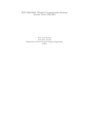
Cordless Telephone System To Connect a Fixed Base Station to a Portable Cordless Handset Early Systems (1980s) have very limited range of few tens of meters [within aHouse Premises] Modern Systems [PACS, DECT, PHS, PCS] can provide a limited range &mobility within Urban CentersCordless HandsetPSTNFixed BaseStation17
Limitations of Simple Mobile Radio Systems The Cellular Approach Divides the Entire Service Area into Several Small Cells Reuse the Frequency Basic Components of a Cellular Telephone System Cellular Mobile Phone: A light-weight hand-held set which is an outcome ofthe marriage of Graham Bell’s Plain Old Telephone Technology [1876] andMarconi’s Radio Technology [1894] [although a very late delivery but verycute] Base Station: A Low Power Transmitter, other Radio Equipment[Transceivers] plus a small Tower Mobile Switching Center [MSC] /Mobile Telephone SwitchingOffice[MTSO] An Interface between Base Stations and the PSTN Controls all the Base Stations in the Region and Processes User ID andother Call Parameters A typical MSC can handle up to 100,000 Mobiles, and 5000 SimultaneousCalls Handles Handoff Requests, Call Initiation Requests, and all Billing &System Maintenance Functions18
19
The Cellular Concept RF spectrum is a valuable and scarce commodity RF signals attenuate over distance Cellular network divides coverage area into cells, each served by its own basestation transceiver and antenna Low (er) power transmitters used by BSs; transmission range determines cellboundary RF spectrum divided into distinct groups of channels Adjacent cells are (usually) assigned different channel groups to avoidinterference Cells separated by a sufficiently large distance to avoid mutual interference canbe assigned the same channel group frequency reuse among co-channelcells20
Cellular Systems: Reuse channels to maximize capacityGeographic region divided into cellsFrequencies/timeslots/codes reused at spatially-separatedlocations. Co-channel interference between same color cells. Base stations/MTSOs coordinate handoff and control functions Shrinking cell size increases capacity, as well as networking burden BASESTATIONMTSO21
Trends in Cellular radio andPersonal Communications PCS/PCN: PCS calls for more personalized services whereas PCN refers toWireless Networking Concept-any person, anywhere, anytime can make a callusing PC. PCS and PCN terms are sometime used interchangeably IEEE 802.11: A standard for computer communications using wirelesslinks[inside building]. ETSI’s 20 Mbps HIPER LAN: Standard for indoor Wireless Networks IMT-2000 [International Mobile Telephone-2000 Standard]: A 3G universal,multi-function, globally compatible Digital Mobile Radio Standard is inmaking Satellite-based Cellular Phone Systems A very good Chance for Developing Nations to Improve their CommunicationNetworks22
UNIT IICELLULAR CONCEPT AND SYSTEMDESIGN FUNDAMENTALS23
2.1 Introduction to Cellular Systems Solves the problem of spectral congestion and user capacity.Offer very high capacity in a limited spectrum without majortechnological changes.Reuse of radio channel in different cells.Enable a fix number of channels to serve an arbitrarily large numberof users by reusing the channel throughout the coverage region.24
Frequency Reuse Each cellular base station is allocated a group of radio channels withina small geographic area called a cell. Neighboring cells are assigned different channel groups. By limiting the coverage area to within the boundary of the cell, thechannel groups may be reused to cover different cells. Keep interference levels within tolerable limits. Frequency reuse or frequency planning seven groups of channel from A to G footprint of a cell - actual radiocoverage omni-directional antenna v.s.directional antenna25
Hexagonal geometry has– exactly six equidistance neighbors– the lines joining the centers of any cell and each of its neighbors areseparated by multiples of 60 degrees. Only certain cluster sizes and cell layout are possible. The number of cells per cluster, N, can only have values which satisfyN i 2 ij j 2 Co-channel neighbors of a particular cell, ex, i 3 and j 2.26
Channel Assignment Strategies Frequency reuse scheme– increases capacity– minimize interference Channel assignment strategy– fixed channel assignment– dynamic channel assignment Fixed channel assignment– each cell is allocated a predetermined set of voice channel– any new call attempt can only be served by the unused channels– the call will be blocked if all channels in that cell are occupied Dynamic channel assignment– channels are not allocated to cells permanently.– allocate channels based on request.– reduce the likelihood of blocking, increase capacity.27
2.4 Handoff Strategies When a mobile moves into a different cell while a conversation is inprogress, the MSC automatically transfers the call to a new channelbelonging to the new base station. Handoff operation– identifying a new base station– re-allocating the voice and control channels with the new base station. Handoff Threshold– Minimum usable signal for acceptable voice quality (-90dBm to -100dBm)– Handoff margin Pr ,handoff Pr ,minimum usablecannot be too large or toosmall.– If is too large, unnecessary handoffs burden the MSC– If is too small, there may be insufficient time to complete handoffbefore a call is lost.28
29
Handoff must ensure that the drop in the measured signal is not dueto momentary fading and that the mobile is actually moving awayfrom the serving base station. Running average measurement of signal strength should be optimizedso that unnecessary handoffs are avoided.– Depends on the speed at which the vehicle is moving.– Steep short term average - the hand off should be made quickly– The speed can be estimated from the statistics of the received short-termfading signal at the base station Dwell time: the time over which a call may be maintained within a cellwithout handoff. Dwell time depends 30
Handoff measurement– In first generation analog cellular systems, signal strength measurementsare made by the base station and supervised by the MSC.– In second generation systems (TDMA), handoff decisions are mobileassisted, called mobile assisted handoff (MAHO) Intersystem handoff: If a mobile moves from one cellular system to adifferent cellular system controlled by a different MSC. Handoff requests is much important than handling a new call.31
Practical Handoff Consideration Different type of users– High speed users need frequent handoff during a call.– Low speed users may never need a handoff during a call. Microcells to provide capacity, the MSC can become burdened if highspeed users are constantly being passed between very small cells. Minimize handoff intervention– handle the simultaneous traffic of high speed and low speed users. Large and small cells can be located at a single location (umbrella cell)– different antenna height– different power level Cell dragging problem: pedestrian users provide a very strong signalto the base station– The user may travel deep within a neighboring cell32
33
Handoff for first generation analog cellular systems– 10 secs handoff time– is in the order of 6 dB to 12 dB Handoff for second generation cellular systems, e.g., GSM––––1 to 2 seconds handoff timemobile assists handoff is in the order of 0 dB to 6 dBHandoff decisions based on signal strength, co-channel interference, andadjacent channel interference. IS-95 CDMA spread spectrum cellular system– Mobiles share the channel in every cell.– No physical change of channel during handoff– MSC decides the base station with the best receiving signal as the servicestation 34
Types of Handoffs: Hard handoff: “break before make” connection Intra and inter-cell handoffsHard Handoff between the MS and BSs35
Cont. Soft handoff: “make-before-break” connection. Mobile directed handoff. Multiways and softer handoffsSoft Handoff between MS and BSTs36
Handoff Prioritization:Two basic methods of handoff prioritization are : Guard Channels Queuing of Handoff37
2.5 Interference and System Capacity Sources of interference––––another mobile in the same cella call in progress in the neighboring cellother base stations operating in the same frequency bandnoncellular system leaks energy into the cellular frequency band Two major cellular interference– co-channel interference– adjacent channel interference38
2.5.1 Co-channel Interference and SystemCapacity Frequency reuse - there are several cells that use the same set offrequencies– co-channel cells– co-channel interference To reduce co-channel interference, co-channel cell must be separatedby a minimum distance. When the size of the cell is approximately the same– co-channel interference is independent of the transmitted power– co-channel interference is a function of R: Radius of the cell D: distance to the center of the nearest co-channel cell Increasing the ratio Q D/R, the interference is reduced. Q is called the co-channel reuse ratio39
For a hexagonal geometryQ D 3NR A small value of Q provides large capacity A large value of Q improves the transmission quality - smaller level ofco-channel interference A tradeoff must be made between these two objectives40
Let i0 be the number of co-channel interfering cells. The signal-tointerference ratio (SIR) for a mobile receiver can be expressed asS ISi0 Iii 1S: the desired signal powerI i: interference power caused by the ith interfering co-channel cellbase station The average received power at a distance d from the transmittingantenna is approximated byor d Pr P0 d0 nclose-in reference pointd0 d P0 :measued power Pr (dBm) P0 (dBm) 10n log d0 n is the path loss exponent which ranges between 2 and 4.TX41
When the transmission power of each base station is equal, SIR for amobile can be approximated asS IR ni0 n D ii 1 Consider only the first layer of interfering cellsS ( D / R)n Ii0 3Ni0 ni0 6 Example: AMPS requires that SIR begreater than 18dB– N should be at least 6.49 for n 4.– Minimum cluster size is 742
For hexagonal geometry with 7-cell cluster, with the mobile unit beingat the cell boundary, the signal-to-interference ratio for the worstcase can be approximated asSR 4 I 2( D R ) 4 ( D R / 2) 4 ( D R / 2) 4 ( D R ) 4 D 443
2.5.2 Adjacent Channel Interference Adjacent channel interference: interference from adjacent infrequency to the desired signal.– Imperfect receiver filters allow nearby frequencies to leak into thepassband– Performance degrade seriously due to near-far effect.receiving filterresponsesignal on adjacent channelsignal on adjacent channeldesired signalFILTERinterferencedesired signalinterference44
Adjacent channel interference can be minimized through carefulfiltering and channel assignment. Keep the frequency separation between each channel in a given cellas large as possible A channel separation greater than six is needed to bring the adjacentchannel interference to an acceptable level. Ensure each mobile transmits the smallest power necessary tomaintain a good quality link on the reverse channel– long battery life– increase SIR– solve the near-far problem45
Trunking and Grade of Service A means for providing access to users on demand from available pool of channels. With trunking, a small number of channels can accommodate large number ofrandom users. Telephone companies use trunking theory to determine number of circuits required. Trunking theory is about how a population can be handled by a limited number ofservers.46
Terminology: Traffic intensity is measured in Erlangs: One Erlang: traffic in a channel completely occupied. 0.5 Erlang: channel occupied30 minutes in an hour. Grade of Service (GOS): probability that a call is blocked (or delayed). Set-Up Time: time to allocate a channel. Blocked Call: Call that cannot be completed at time of request due to congestion.Also referred to as Lost Call. Holding Time: (H) average duration of typical call. Load: Traffic intensity across the whole system. Request Rate: (λ) average number of call requests per unit time.47
Traffic Measurement (Erlangs)48
49
50
51
52
53
54
55
Erlang C Model –Blocked calls cleared A different type of trunked system queues blocked calls –Blocked CallsDelayed. This is known as an Erlang C model. Procedure: Determine Pr[delay 0] probability of a delay from the chart. Pr[delay t delay 0 ] probability that the delay is longer than t, giventhat there is a delay Pr[delay t delay 0 ] exp[-(C-A)t /H ] Unconditional Probability of delay t : Pr[delay t ] Pr[delay 0] Pr[delay t delay 0 ] Average delay time D Pr[delay 0] H/ (C-A)56
Erlang C Formula The likelihood of a call not having immediate access to a channel is determinedby Erlang C formula:57
58
59
60
2.7 Improving Capacity in Cellular Systems Methods for improving capacity in cellular systems– Cell Splitting: subdividing a congested cell into smaller cells.– Sectoring: directional antennas to control the interference and frequencyreuse.– Coverage zone : Distributing the coverage of a cell and extends the cellboundary to hard-to-reach place.61
Cell Splitting Cell Splitting is the process of subdividing the congested cell into smallercells (microcells),Each with its own base station and a correspondingreduction in antenna height and transmitter power. Cell Splitting increases the capacity since it increases the number of timesthe channels are reused.62
2.7.1 Cell Splitting Split congested cell into smaller cells.– Preserve frequency reuse plan.– Reduce transmission power.Reduce R to R/2microcell63
Illustration of cell splitting within a 3 km by 3 km square64
Transmission power reduction from Pt1 to Pt 2 Examining the receiving power at the new and old cell boundaryPr [at old cell boundary ] Pt1 R nPr [at new cell boundary ] Pt 2 ( R / 2) n If we take n 4 and set the received power equal to each otherPt116 The transmit power must be reduced by 12 dB in order to fill in theoriginal coverage area. Problem: if only part of the cells are splitedPt 2 – Different cell sizes will exist simultaneously Handoff issues - high speed and low speed traffic can besimultaneously accommodated65
2.7.2 Sectoring Decrease the co-channel interference and keep the cell radius Runchanged– Replacing single omni-directional antenna by several directional antennas– Radiating within a specified sector66
Interference Reductionposition of themobileinterference cells67
2.7.3 Microcell Zone Concept Antennas are placed at the outer edges of the cell Any channel may be assigned to any zone by the base station Mobile is served by the zone with the strongest signal. Handoff within a cell– No channel reassignment– Switch the channel to adifferent zone site Reduce interference– Low power transmittersare employed68
Multiple Access Techniques for WirelessCommunication:Many users can access the at same time, share a finite amount of radio spectrum withhigh performance duplexing generally required frequency domain time domain. Theyaccessing techniques are, FDMA TDMA SDMA PDMA69
Frequency division multiple access FDMA One phone circuit per channel Idle time causes wasting of resources Simultaneously and continuously transmitting Usually implemented in narrowband systems For example: in AMPS is a FDMA bandwidth of 30 kHz implemented70
Time Division Multiple Access Time slots One user per slot Buffer and burst method Noncontinuous transmission Digital data Digital modulation71
Features of TDMA A single carrier frequency for several users Transmission in bursts Low battery consumption Handoff process much simpler FDD : switch instead of duplexer Very high transmission rate High synchronization overhead Guard slots necessary72
Space Division Multiple Access Controls radiated energy for each user in space using spot beam antennas base station tracks user when moving cover areas with same frequency: TDMA or CDMA systems cover areas with same frequency: FDMA systems73
Space Division Multiple Access primitive applications are“Sectorizedantennas” In future adaptive antennas simultaneouslysteer energy in the direction of many users atonce74
UNIT IIIMOBILE RADIO PROPAGATION75
. Mobile Radio Propagation RF channels are random – do not offer easy analysis difficult to model – typically done statistically for a specific systemIntroduction to Radio Wave Propagation: diverse mechanismsof electromagnetic (EM) wave propagation generally attributed to(i) diffraction(ii) reflection(iii) scattering non-line of sight (NLOS – obstructed) paths rely on reflections obstacles cause diffraction multi-path: EM waves travel on different paths to a destination –interaction of paths causes fades at specific locations76
traditional Propagation Models focus on(i) transmit model - average received signal strength at given distance(ii) receive model - variability in signal strength near a given location(1) Large Scale Propagation Models: predict mean signal strengthfor TX-RX pair with arbitrary separation useful for estimating coverage area of a transmitter characterizes signal strength over large distances (102-103 m) predict local average signal strength that decreases withdistance77
(2) Small Scale or Fading Models: characterize rapid fluctuations ofreceived signal over short distances (few ) or short durations (few seconds)with mobility over short distances instantaneous signal strength fluctuates received signal sum of many components from different directions phases are random sum of contributions varies widely received signal may fluctuate 30-40 dB by moving a fraction of 78
Large-scale small-scale propagation79
Reflection Perfect conductors reflect with no attenuation– Like light to the mirror Dielectrics reflect a fraction of incident energy– “Grazing angles” reflect max*– Steep angles transmit max*– Like light to the waterq Reflection induces 180 phase shiftqrqt– Why? See yourself in the mirror80
Classical 2-ray ground bounce model One line of sight and one ground bound81
Method of image82
Vector addition of 2 rays83
Simplified modelht2 hr2Pr Pt Gt Gr 4d Far field simplified modelExample 2.284
Diffraction Diffraction occurs when waves hit the edge of an obstacle– “Secondary” waves propagated into the shadowed region– Water wave example– Diffraction is caused by the propagation of secondary waveletsinto a shadowed region.– Excess path length results in a phase shift– The field strength of a diffracted wave in the shadowed region isthe vector sum of the electric field components of all thesecondary wavelets in the space around the obstacle.– Huygen’s principle: all points on a wavefront can be consideredas point sources for the production of secondary wavelets, andthat these wavelets combine to produce a new wavefront in thedirection of propagation.85
Diffraction geometry Fresnel-Kirchoff distraction parameters,86
Fresnel Screens Fresnel zones relate phase shifts to thepositions of obstacles A rule of thumb used for line-of-sightmicrowave links 55% of the first Fresnel zone iskept clear.87
Knife-edge diffraction loss Gain88
Scattering Rough surfaces– Lamp posts and trees, scatter all directions– Critical height for bumps is f( ,incident angle),– Smooth if its minimum to maximum protuberance h is lessthan critical height.– Scattering loss factor modeled with Gaussian distribution, Nearby metal objects (street signs, etc.)– Usually modeled statistically Large distant objects– Analytical model: Radar Cross Section (RCS)– Bistatic radar equation,89
Impulse Response Model of a Time Variant MultipathChannel90
3.2 Free Space Propagation Modelused to predict signal strength for LOS path satellites LOS uwave power decay d –n (d separation)Subsections(1) Friis Equation(2) Radiated Power(3) Path Loss(4) Far Field Region91
(1) Friis free space equation: receive power at antenna separated bydistance d from transmitterPr(d) Gt Gr 2 Pt 2 2 ( 4 ) L d(3.1)Pr & Pt received & transmitted powerGt & Gr gain of transmit & receive antenna wavelengthd separationL system losses (line attenuation, filters, antenna)- not from propagation- practically, L 1, if L 1 ideal system with no losses power decays by d 2 decay rate 20dB/decade92
Antenna GainG 4 Ae2 (3.2) Ae effective area of absorption– related to antenna sizeAntenna Efficiencyη Ae/AA antenna’s physical area (cross sectional) for parabolic antenna η 45% - 50% for horn antenna η 50% - 80%93
(2) Radiated PowerIsotropic Radiator: ideal antenna (used as a reference antenna) radiates power with unit gain uniformly in all directions surface area of a sphere 4πd 2 2Effective Area of isotropic antennae given by Aiso 4 2 1 2 P PTIsotropic Received Power PR 22 T 4 d 4 4 d d transmitter-receiver separationPT 4 d PR 22Isotropic free space path lossLp f 2 relationship with antenna size results from dependence of Aiso on 94
Directional Radiationpractical antennas have gain or directivity that is a function of θ azimuth: look angle of the antenna in the horizontal plane elevation: look angle of the antenna above the horizontal plane Let Φ power flux desnityθtransmit antenna gain is given by:GT(θ, ) Φ in the direction of (θ, )Φ of isotropic antennareceive antenna gain is given by:GR(θ, ) Ae in the direction of (θ, )Ae of isotropic antenna95
Principal Of Reciprocity: signal transmission over a radio path is reciprocal the locations of TX & RX can be interchanged without changingtransmission characteristicssignals suffers exact same effects over a path in either direction in aconsistent order implies that GT(θ, ) GR(θ, )thus maximum antenna gain in either direction is given byAe4 AeG 2Aiso 96
EIRP: effective isotropic radiated power represents maximum radiated power available from a transmitter measured in the direction of maximum antenna gain as compared toisotropic radiatorEIRP PtGiso(3.4)ERP: effective radiated power - often used in practice denotes maximum radiated power compared to ½ wave dipoleantenna dipole antenna gain 1.64 (2.15dB) isotropic antenna thus EIRP will be 2.15dB smaller than ERP for same systemERP PtGdipole97
1. Outdoor Propagation Models–––––1.1 Longley-Rice Model1.2 Okumura Model1.3. Hata Model1.4. PCS Extension to Hata Model1.5. Walfisch and Bertoni Model98
Outdoor Propagation Models Propagation over irregular terrain. The propagation models available forpredicting signal strength vary very widely intheir capacity, approach, and accuracy.99
Longley-Rice Model also referred to as the ITS irregular terrainmodel frequency range from 40 MHz to 100 GHz Two version: point-to-point using terrain profile. area mode estimate the path-specificparameters100
Okumura Model Frequency range from150 MHz to 1920 MHz BS-MS distance of 1 km to 100 km. BS antenna heights ranging from 30 m 1000 m.L 50 ( dB ) L f Amu ( f , d ) G ( hte ) G ( hre ) G AREA Lf is the free space propagation loss, Amu is the median attenuation relative to free space, G(tte ) is the base station antenna height gain factor, G(tre ) isthe mobile antenna height gain factor, GAREA is the gain due to the type of environment.101
Hata Model Frequency range from150 MHz to 1500 MHz BS-MS distance of 1 km to 100 km. BS antenna heights ranging from 30 m 200 m.L 50 (urban) dB 69.55 26.16 log f c 13.82 log hte a hre 44.9 6.55 log hte log d fc is the frequency (in MHz) from 150 MHz to 1500 MHz,hte is the effective transmitter antenna height (in meters)hre is the effective receiver (mobile) antenna height (1.10 m)d is the T-R separation distance (in km),a(hre ) is the correction factor for effective mobile antennaheight (large city, small to medium size city, suburban, openrural)102
PCS Extension to Hata Model Frequency range from1500 MHz to 2000 MHz BS-MS distance of 1 km to 20 km. BS antenna heights ranging from 30 m 200 m.L50 urban 46.3 33.9 log f c 13.82 log hte a hre 44.9 6.55 log hte log d C Mfc is the frequency (in MHz) from 1500 MHz to 2000 MHz,hte is the effective transmitter antenna height (in meters)hre is the effective receiver (mobile) antenna height (1.10 m)d is the T-R separation distance (in km),a(hre ) is the correction factor
In 1934,AM mobile communication systems for municipal police radio systems. Vehicle ignition noise was a major problem. In 1946, FM mobile communications for the first public mobile telephone service Each system used a single, high-powered tran