Transcription
Real-time water renderingIntroducing the projected grid conceptMaster of Science thesisClaes Johanson claes@vember.net March 2004Lund UniversitySupervisor:Calle LejdforsDepartment of Computer Science, Lund UniversityThe thesis was done in cooperation withSaab Bofors DynamicsSupervisor at SBD: Magnus Anderholm, RTLI
AbstractThis thesis will examine how a large water surface can be rendered in an efficient manner using moderngraphics hardware. If a non-planar approximation of the water surface is required, a high-resolutionpolygonal representation must be created dynamically. This is usually done by treating the surface as aheight field. To allow spatial scalability, different methods of “Level-Of-Detail” (LOD) are often usedwhen rendering said height field. This thesis presents an alternative technique called “projected grid”. Theintent of the projected grid is to create a grid mesh whose vertices are even-spaced, not in world-spacewhich is the traditional way but in post-perspective camera space. This will deliver a polygonalrepresentation that provides spatial scalability along with high relative resolution without resorting tomultiple levels of detail.
ContentsContentsAbstract .3Contents .51Background.71.1Introduction .71.2The graphics pipeline.71.3Height-fields.81.4Task subdivision.91.5Tessellation schemes.91.6Generating waves. 101.7The optics of water . 111.2.11.2.22Projected Grid . 112.1Concept. 112.2Definitions . 112.3Preparation . 112.4The proposed algorithm . 112.5Further restriction of the projector . 112.3.12.3.22.3.32.4.12.4.23A real-world analogy . 11The projector matrix . 11What can possibly be seen?. 11Aiming the projector to avoid backfiring. 11Creating the range conversion matrix. 11Implementation . 113.1Implementation suggestions . 113.2Height-map generation . 113.3Rendering additional effects into the height-map . 113.4Shading . 113.5Proposed solutions for reducing overdraw . .73.4.83.5.13.5.23.5.34Overview. 7Vertex transformations . 8CPU-based vertex-processing. 11GPU-based vertex-processing using render-to-vertexbuffers. 11CPU-based vertex-processing with GPU based normal-map generation. 11The view-vector . 11The reflection vector. 11The Fresnel reflectance term . 11Global reflections . 11Sunlight . 11Local reflections. 11Refractions. 11Putting it all together. 11Patch subdivision. 11Using scissors. 11Using the stencil buffer. 11Evaluation . 11-5-
Contents4.1Implications of the projected grid . 114.2Future work . 114.3Conclusion . 11Appendix A - Line - Plane intersection with homogenous coordinates . 11Appendix B - The implementation of the demo application . 11Appendix C – Images. 11Terms used. 11References . 11-6-
Background1 Background1.1 IntroductionThe process of rendering a water surface in real-time computer graphics is highly dependent on thedemands on realism. In the infancy of real-time graphics most computer games (which is the primaryapplication of real-time computer graphics) treated water surfaces as strictly planar surfaces which hadartist generated textures applied to them. The water in these games did not really look realistic, but neitherdid the rest of the graphics so it was not particularly distracting. Processing power were (by today’sstandard) quite limited back then so there were not really any alternatives. But as the appearance of thegames increase with the available processing power, the look of the water are becoming increasinglyimportant. It is one of the effects people tend to be most impressed with when done right.Water rendering differ significantly from rendering of most other objects. Water itself has severalproperties that we have to consider when rendering it in a realistic manner: It is dynamic. Unless the water is supposed to be totally at rest it will have to be updated each frame.The wave interactions that give the surface its shape are immensely complex and has to beapproximated. The surface can be huge. When rendering a large body of water such as an ocean it will often span allthe way to the horizon. The look of water is to a large extent based on reflected and refracted light. The ratio between thereflected and refracted light vary depending on the angle the surface viewed at.It is necessary to limit the realism of water rendering in order to make an implementation feasible. In mostgames it is common to limit the span of the surface to small lakes and ponds. The wave interactions arealso immensely simplified. As mentioned in the introductory example, the reflections and refractions areusually ignored, the surface is just rendered with a texture that is supposed to look like water. Neither is ituncommon that water still is treated as a planar surface without any height differences whatsoever. But thestate of computer generated water is rapidly improving and although most aspects of the rendering still arecrude approximations they are better looking approximations than the ones they replace.The remainder of this chapter will give a brief overview of how water rendering could be implemented.1.2 The graphics pipeline1.2.1 OverviewReal-time three-dimensional computer graphics is a field of technology that have matured substantiallyduring the last decade. The mid 1990’s saw the introduction of hardware accelerated polygonal scan-linerendering aimed at the consumer market. This allowed applications to offload the CPU by moving certaingraphics-related operations to the graphics hardware. At first only the pixel processing were handled bythe hardware but after a while the hardware started to support vertex processing as well. A problem withthe graphics pipeline at this stage was that its functionality was fixed. It was possible to alter some states tocontrol its behaviour but it could not do anything it was not built to do. The last two hardwaregenerations, as of writing, (which support the features added by DirectX 8 and 9 [1]) have replaced thisfixed function pipeline with programmable units at key locations, giving a somewhat CPU-like freedomwhen programming. The latest generation added floating-point capabilities and a significantly increasedinstruction count to the pixel-pipeline as well, making it even more generic. Although the programmabilityhas increased, the basic data flow is still hardwired for use as a scan-line renderer.-7-
BackgroundVertexDataVertexShadersViewportsand textureGeometry pipelineAlpha, Stencil andDepth-TestingFrame BufferBlendingPixel and TextureBlendingRasterizationFigure 1.1 Overview of the DirectX 8 pipeline1.2.2 Vertex transformationsThe traditional vertex transformation used to transform the vertex data from its original state intocoordinates on the screen will vary depending on implementation. The principle is that there are severalspaces which geometry can be transformed between using 4x4 matrices.In this thesis the matrix notations from DirectX 9 [1] will be used with the exception that ‘projectedspace’ will be referred to as ‘post-perspective space’ to avoid confusion. A left-handed coordinate systemis erspectivePost-perspectivespaceFigure 1.2 Matrix notation used in the thesis.The camera frustum is defined as the volume in which geometry has the potential to be visible by thecamera. It is often useful to see a geometric representation of the camera frustum. This can beaccomplished by taking its corner points ( 1, 1, 1) defined in post-perspective space and transformthem to world-space.1.3 Height fieldsA water body can be represented as a volume. For every point within this volume we are able to tellwhether it is occupied by water or not. But all this information is superfluous, as we really only need toknow the shape of the surface (the boundary between the water body and the surrounding air) in order torender it. This surface can often be simplified further to a height field (fHF). A height field is a function oftwo variables that return the height for a given point in two-dimensional space. Equation 1.1 show how aheight field can be used to displace a plane in three-dimensional space.pheightfield (s, t ) p plane (s, t ) f HF (s, t ) N planeEquation 1.1Using a height field as a representation for a water surface does have its restrictions compared to a generalsurface. As the height field only represent a single height-value for each point it is impossible to have onepart of the surface that overlap another. Figure 1.3 shows a two-dimensional equivalent of the limitationwhere the right image cannot represent the part of the curve that overlap.-8-
BackgroundyyxxFigure 1.3 Illustrations of the limitations that apply to height fields. (2D equivalent)left: (x,y) (fx[s], fy[s])right: (x,y) (x, f[x])The height field has many advantages as it is easy to use and it is easy to find a data structure that isappropriate for storing it. It is often stored as a texture, which is called height map. The process ofrendering a surface with height map is usually called displacement-mapping as the original geometry (Pplanein Equation 1.1) is displaced by the amount defined in the height map.The rest of this thesis will only deal with rendering height fields and not discuss more general surfaces.1.4 Task subdivisionAs hardware is built with scan-line rendering in mind there is no way to get around that the surface musthave a polygonal representation. Thus we need to approximate the surface with some kind of grid (notnecessarily regular). As a height field representation will be used it is appropriate to generate a planar gridfirst, and then displace the points afterwards.We can divide the water rendering task into these subtasks:1. Generate the planar grid (tessellation schemes)2. Generate the height field and sample the points in the grid3. Render and shade the resulting geometryStep 1 and 2 are not strictly separate as the generation of height-data may impose certain restrictions onhow the grid must be generated. Neither do they have to be separate in an implementation. But it is goodto treat them as separate tasks from an explanatory point of view.1.5 Tessellation schemesA surface of water is continuous in real life as far as we are concerned. But interactive computer graphicsneed a polygonal representation so the surface must be discretized. A tessellation scheme is the process ofdetermining in which points the height field should be sampled.The most straightforward way to represent a surface is to draw it as a rectangular regular grid in worldspace.The grid has a detail-level that is constant in world-space. But due to the perspective nature of theprojective part of the camera-transform (MPerspective) through which the geometry is rendered, the detail-levelin the resulting image will be dependant on the distance to the viewer. While this might work for a smallsurface like a lake or a pond, it will not be suitable in a scene where an ocean is supposed to cover theentire screen along with a horizon that is far away. The grid would have to be spread over such a largearea that the resulting points in the grid would be too sparse to represent the level of detail we want.The perspective effect have the implication that we can see both parts of the surface that are close, andparts of the surface that are distant simultaneously. In this thesis the distance between the nearest visiblepoint on the surface to the most distant visible point will be referred to as distance dynamic range. Asingle rectangular grid is good when the dynamic range is small, but for large dynamic ranges, a moresophisticated solution is required.A common solution is to use what is known as a LOD (level-of-detail) scheme. The surface is divided intoa grid of patches. When rendering, the resolution of each patch will be determined by the distance to theviewer. The change in resolution is discrete and each level-of-detail usually has twice the resolution of the-9-
Backgroundprevious one. There are many well developed implementations that are used for height map rendering thatderives from the LOD concept which are used for landscape rendering. However, most of them rely onpre-processing to a certain amount. When using pre-processing, each patch does not even have to be aregular grid but can contain any arbitrary geometry as long as it matches the adjacent patches at the edges.However, as water is dynamically generated each frame that makes no sense to rely on any pre-processingall.Figure 1.4 shows a suggestion how LOD could be used for water rendering. The suggested approach issimilar to geomipmapping [6] with the exception that the level determination has been simplified. (EachLOD level has a constant parameter d whereas geomipmapping uses pre-processing to determine d. Whenthe viewer is closer than d a LOD level switch occurs.)Figure 1.4 Illustration of the LOD concept. The grid gets sparser further away from the camera.The implementation of this LOD-scheme is pretty straightforward. For all potentially visible patches,determine the level of detail depending on the distance between the patch and the camera, sample theheight-data for the points in the patch and render the resulting patch.The LOD-concept is not without difficulties though, as level-switches can cause a couple of artefacts.With a moving camera patches will frequently change level, causing a ‘pop’. The pop occurs because thenew detail level will look slightly different than the previous one (due to having more/less detail). As theswitch is instantaneous it is often rather noticeable. There will also be discontinuities between patches ofdiffering detail-levels (see the white arrow in Figure 1.4, the middle point to the left can have a differentheight than the interpolated value to the right.). This is usually solved by rendering a so-called “skirt” atthe edges between detail-level boundaries and/or to interpolate between the detail-levels to make theswitch continuous. The solutions to these issues are mentioned in far more detail in [6] but that is outsidethe scope of this thesis.Chapter 2 will introduce a new tessellation-scheme called projected grid that is appropriate for waterrendering.1.6 Generating wavesThere are a number of different approaches to choose from when generating the height-data for adisplaced surface.The Navier-Stokes Equations (NSE) is the cornerstone in the field of Fluid Mechanics and is defined by aset of differential equations that describe the motion of incompressible fluids. The NSEs are complexbeasts, but they can be simplified and discretized to something we can use. In [7] it is suggested that arectangular grid of columns are used to represent the volume of the water body. For every column, a setof virtual pipes are used to describe the flow of fluid between itself and the adjacent columns.- 10 -
BackgroundFigure 1.5 Approximation of the NSE. The images are copied from [7].Although they are extremely realistic, the NSEs are somewhat impractical for our intended use. Theyrequire a world space grid to be calculated every frame and that grid cannot be big enough to cover anentire sea with enough detail. As the previous state of the surface has to be known, it is also hard tocombine this with tessellation schemes that dynamically change their tessellation depending on theposition of the viewer. Since the entire process of wind building up the momentum of waves has to besimulated it is unsuitable to open-water waves. A real-time implementation will have to be limited tosmaller local surfaces. It is certainly useful in combination with another wave model. That way the NSEonly have to take care of the water’s response to objects intersecting it, and only at local areas.With the purpose of rendering large water bodies, it is more practical to have a statistical model ratherthan simulating the entire process of the waves being built up. Oceanographers have developed modelsthat describe the wave spectrum in frequency domain depending on weather conditions. These spectrumscan be used to filter a block of 2D-noise by using the Fourier transform. This method can be acomputationally efficient way to generate a two-dimensional height map. This is explained in more detailin [4].The method that was used for the demo implementations in this thesis is a technique called Perlin noise([5] named after Ken Perlin) which gives a continuous noise. To generate Perlin noise it is required tohave a reproducible white noise (a noise which can be accessed multiple times with the same value as theresult). This can either be generated by storing white noise in memory or by using a reproducible randomfunction. Perlin noise is obtained by interpolating the reproducible noise. Given the right interpolator,Perlin noise will be continuous. The basic Perlin noise does not look very interesting in itself but bylayering multiple noise-functions at different frequencies and amplitudes a more interesting fractal noisecan be created. The frequency of each layer is usually the double of the previous layer which is why thelayers usually are referred to as octaves. By making the noise two-dimensional we can use it as a texture.By making it three-dimensional we can animate it as well.Figure 1.6 Multiple octaves of Perlin noise sums up to a fractal noise. (α 0.5)In Figure 1.6 it can be seen how the sum of multiple octaves of Perlin noise result in a fractal noise. Thecharacter of the noise will depend on the amplitude relationship between successive octaves of the noise.fnoise( x) octaves 1 αi noise(2i x)Equation 1.2i 0- 11 -
BackgroundEquation 1.2 demonstrates how a fractal noise can be created from multiple octaves of Perlin noise andhow all the amplitudes can be represented by a single parameter (α). Higher values for α will give arougher looking noise whereas lower values will make the noise smoother.1.7 The optics of waterTo render a water surface in a convincing manner, it is important to understand how light behaves whenwe look at water in reality. Water itself is rather transparent, but it has a different index-of-refraction(IOR) than air which causes the photons that pass the boundaries between the mediums to get eitherreflected or transmitted (see Figure 1.7).Incoming lightNormalθiReflected lightθrn1Airn2WaterθtTransmitted lightFigure 1.7 Light transport through a air/water-boundary.The angles θ i and θ t can be obtained from Snell’s law (assuming θ i θ1 , θt θ 2 ):n1 sin (θ1 ) n 2 sin (θ 2 )Equation 1.3Snell’s law is used to calculate how θ i differs from θ t depending on n1 and n2 which are the IORs of thetwo mediums.The look of water depends greatly on the angle with which we view it. When looking straight down intothe water we can easily see what’s beneath the surface as long as the water itself is clear. But when lookingtowards the horizon it will almost act as a mirror. This phenomenon was studied by Augustin-Jean Fresnelwhich resulted in the Fresnel equations [2] which allows the reflection coefficient (the probability that aphoton is reflected) to be calculated. As the light in most cases is non-polarized the reflection coefficientcan be described as:2 sin(θ i θ t ) tan(θ i θt ) R sin(θi θt ) tan(θi θ t ) 2Equation 1.4The transmission coefficient (the probability that a photon is transmitted across the boundary into thenew medium) is given by:T (1 R )Equation 1.5- 12 -
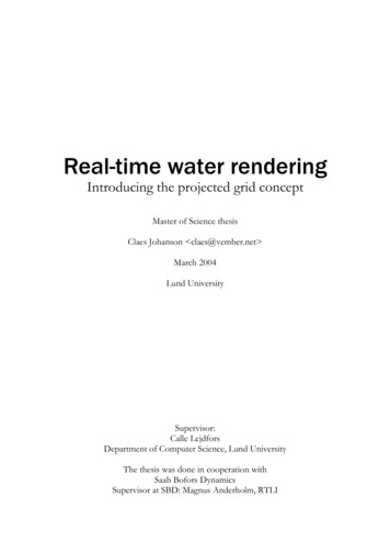
BackgroundIn Figure 1.8 it can be seen graphically how this apply to the water air boundary.reflection coefficientair - water refractionwater - air refraction110.80.80.60.60.40.40.20.2003060angle of incidence (degrees)09003060angle of incidence (degrees)90Figure 1.8 Fresnel reflection coefficient for the air water boundaryThe IOR of water is dependent on several properties including the wavelength of the light, thetemperature of the water and its mineral content. The documented IOR of sweet water at 20 C accordingto [4] is:wavelengthIOR at 20 C700 nm (red)1.33109530 nm (green)1.33605460 nm (blue)1.33957As can be seen the differences are quite insignificant, and all three values could be approximated with asingle value without any obvious degradation in realism. In fact, when quantitized to three 8-bit values(with the intention of using it as a texture lookup), the three values never differed from each other morethan by a value of 1. This was true both in linear colour space and sRGB (the standard windows colourspace with a gamma of 2.2). It is safe to assume that all of these variations can be ignored for ourpurposes as it is unlikely they will ever cause any noticeable difference.Figure 1.9 Implication of the Fresnel reflectance term. The left image shows a photo of the Nile where youcan see the reflectance vary depending on the normal of the surface. The right image shows a computergenerated picture where the Fresnel reflectance for a single wavelength is output as a grey-scale (white fully reflective, black fully refractive).- 13 -
Projected Grid2 Projected Grid2.1 ConceptThe projected grid concept was developed with the desire of having a tessellation scheme that wouldgenerate a geometric representation of a displaced surface that as closely as possible matched a uniformgrid in post-perspective space. What we’re going to do is to take the desired post-perspective space gridand run it backwards through the camera’s view and perspective transforms.The “naïve” projected grid algorithm: Create a regular discretized plane in post-perspective space that is orthogonal towards the viewer. Project this plane onto a plane in world-space (Sbase). Displace the world-space vertices according to the height field (fHF). Render the projected planeWithout displacement the plane would, when rendered, result in the same plane that was created at thefirst step of the algorithm (as seen from the viewer). The depth coordinates will be different though.The ability to displace the coordinates in world-space is the whole purpose of the projected grid.Figure 2.1 Simple non-displaced projected gridThe full projected grid algorithm is given in section 2.4. But to make it easier to understand (and motivate)the full algorithm we will showcase what makes the naïve algorithm unsuitable for general use in section2.3.2.2 DefinitionsThese are the definitions used in this chapter.Notation used:p - point in homogenous three-dimensional spaceM - 4x4 matrixS - planeN - normalV - volume- 14 -
Projected GridNbaseVdisplaceablefHFSupperSbaseSlowerFigure 2.2 2D illustration of the definitionsBase plane: SbaseThe plane that define the non-displaced placement of the grid in world-space. It is defined by its origin(pbase) and its normal (Nbase). The points in the grid will be displaced along the normal of the plane, with thedistance depending on the height field function (fHF).Height field function: fHF(u,v)Given surface coordinates u and v, it returns the value of the height field at that position.Upper/Lower bound: Supper, SlowerIf the entire surface is displaced by the maximum amount upwards then the resulting plane defines theupper bound (Supper). The lower bound (Slower) is equivalent but in the downward direction.Together the planes define the allowed range of displacement.pupper pbase Nbase max( f HF ) , Nupper Nbaseplower pbase Nbase min ( f HF ) , Nlower NbaseEquation 2.1 Definition of the upper/lower bound planes. (Assuming that Nbase is of unit length.)Displaceable volume: VdisplaceableThe volume between the upper and lower bounds.Camera frustum: VcamThe frustum of the camera for which the resulting geometry is intended to be rendered by.Visible part of the displaceable volume: VvisibleThis is the intersection of Vdisplaceable and Vcam.2.3 PreparationThis section is intended to highlight some of the issues that plague the naïve algorithm. The properprojected grid algorithm (as described in section 2.4) will overcome these issues but it is crucial to have anunderstanding of
The process of rendering a water surface in real-time computer graphics is highly dependent on the demands on realism. In the infancy of real-time graphics most computer games (which is the primary application of real-time computer graphics) treated water surfaces as strictly planar surf