WIXLIB

FREQUENCY COUPLING IN VISUAL AND AGRANULAR CORTEXData were collected with a 24-channel linear microelectrode array(Plexon U-Probe, Plexon, Dallas, TX), with an interelectrode spacingof 100 m (V1 recordings) or 150 m (SEF recordings). The range ofimpedance measured for all channels was 0.3– 0.5 M at 1 kHz. Afterinserting the linear microelectrode array into the target chamber at thedesired depth, we waited 1– 4 h until the recorded data indicated thatthe electrode had reached a stable position in cortex. After theelectrode had stabilized, we recorded 7– 60 min of resting-state LFP innear-total darkness with the monitor powered off. Extracellular voltages were measured over time in reference to the electrode shaft. ForV1 recordings, the data were amplified and filtered in the range of 0.3Hz–7.5 kHz, digitized at 30 kHz, and stored with the BlackrockMicrosystems Cerebus system (Salt Lake City, UT). V1 LFP wasextracted off-line by filtering the broadband data between 0.5 Hz and500 Hz and decimating by a factor of 30, resulting in a sampling rateof 1 kHz. For SEF recordings, all data were streamed with the PlexonMAP system (Plexon). SEF LFP data were computed by band-passfiltering between 0.2 and 300 Hz and amplifying with a gain of 1,000,followed by digitizing at 1 kHz.Experimental conditions. The main focus of this study is on datacollected during the resting state. However, each day we also presented full-screen visual flashes in order to assess the depth of theelectrode in cortex (see Laminar electrode placement). For V1, aflashing white light stimulus was produced with MonkeyLogic 1.2(Asaad and Eskandar 2008) in MATLAB 2011b (32 bit) running on aPC with Windows 7 (64 bit) using an NVIDIA GeForce GTX 680graphics board. The stimulus filled the entire screen (45 27 ). Inthis passive viewing paradigm, the animal was presented with periodic50-ms flashes of white light (luminance of 74.7 cd/m2 in CIE colorspace), each followed by a 1-s black blank (0.470 cd/m2) screen for aperiod of 20 min. For SEF sessions, when the monkey’s gaze fellwithin 11 of the center of the CRT monitor a white square (34.8cd/m2, 14.3 ms at 70 Hz) was presented for a single frame (14.3 ms)at the central area of the CRT monitor (corresponding to the central40 36 of the visual field), followed by 500 ms of a blank blackscreen (0.1 cd/m2) for as long as the monkey’s gaze remained in thiscentral window. The stimulus presentation was provided in blocks of100 –200 presentations. Flash presentation and eye position monitoring were performed by dedicated computers (TEMPO, ReflectiveComputing, Olympia, WA; EyeLink, SR Research, Mississauga, ON,Canada). The timing of visual light flashes was measured by aphotodiode positioned against the monitor.Laminar electrode placement. Accurate laminar placement of theelectrode channels was required for these experiments. This wasachieved through multiple steps, checks, and tests (Fig. 1).1) The linear microelectrode arrays were inserted slowly. Uponpenetration of the dura mater, the depth of the electrode array in cortex(usually just a few hundred micrometers) was discerned by contrasting the 1/f (pink) noise profile of the neural LFP on array channelsin neuropil from the Gaussian noise profile on channels outside of thebrain (Fig. 1E). The array of channels was never fully advanced intothe cortex in order to identify the depth of cortical entry. If a guidetube was used to fortify the electrode during penetration, it wasretracted after the array entered the brain to ensure that no channelswere occluded. Note that no penetration through the dura mater wasmade with a guide tube.2) The distinction between channels inside and outside the neocortex was validated by the presence of spontaneous and visually evokedsingle-unit and multiunit spiking activity.3) Converging evidence for array depth was obtained from thelaminar profile of LFP gamma power (40 – 80 Hz), which is quantifiably attenuated on channels outside the cortex. Gamma power istypically increased in middle layers and decreased in lower layers inboth V1 (Maier et al. 2010; Smith et al. 2013; Xing et al. 2012) andSEF (Godlove et al. 2014).32434) Further converging evidence for array depth in V1 was obtainedfrom a clear separation of LFP coherence between L4C and L5 (Maieret al. 2010).5) Further converging evidence for array depth in SEF was obtained from the laminar profile of spike width, corresponding to thehistological distribution of pyramidal cells and interneurons (Godloveet al. 2014).6) Further converging evidence for array depth was provided by thedistinctive laminar profile of the visually evoked CSD in V1 (Hansenet al. 2012; Kajikawa and Schroeder 2011; Schroeder et al. 1998; Selfet al. 2013) and in SEF (Godlove et al. 2014) (Fig. 1F). This approachis detailed in the next section.7) Further converging evidence for proximity to the pial surfacewas marked by a commonly observed electrocardiogram signal (Godlove et al. 2014) (Fig. 1F).8) These neurophysiological criteria were supplemented with several imaging techniques to verify both cortical penetration depth andorthogonality of the electrode to the cortical surface with highresolution MRI (Maier et al. 2008) and a combination of CT scans andMRI (Godlove et al. 2014) (Fig. 1, A–D).Previous work has established that similar criteria for matchingpenetration depth and distinction of laminar compartments correspondto the position of deliberately placed electrolytic lesions when verifiedin histological sections (Schroeder et al. 1998).Intersession alignment of laminar data. Each recording sessionresulted in time-varying voltage from each of the 24 electrode channels. To average data aligned for cortical depth of the array acrosssessions, we employed CSD analysis of visual responses to briefflashes of light (Maier et al. 2010; Fig. 1F). After constructingevent-related LFPs, triggering to the onset of each flash, and averaging across samples, we calculated the second spatial derivative definedby a three-point formula:CSD X共t, c z兲 2X共t, c兲 X共t, c z兲z2where X is the extracellular voltage recorded in microvolts at time tfrom an electrode channel at position c and z is the electrode interchanneldistance (100 m for V1 recordings and 150 m for SEF recordings)(Nicholson and Freeman 1975). To convert this measure into units ofcurrent per unit volume, we multiplied the result by an estimate of theconductivity of cortex, 0.4 S/m (Logothetis et al. 2007).The location of granular L4C in V1 is uniquely characterized by anearly current sink, reflecting the excitatory postsynaptic potentialsproduced by geniculate activation (Mitzdorf and Singer 1979). Weidentified the channel positioned at the bottom of this initial currentsink, typically located 0.8 –1.3 m below the dura, and aligned arraydepths across sessions on this reference point (Maier et al. 2010). Datafrom SEF were aligned with an automated approach that finds theoptimum depth estimates by minimizing the summed differencesbetween every CSD profile in the data set (Godlove et al. 2014).Data analysis. Data analyses were performed in MATLAB (R2013a,MathWorks, Natick, MA) with custom-written scripts and with theFieldTrip toolbox (Oostenveld et al. 2011). Analyses in this reportparallel precisely and extend those described in Spaak et al. (2012).Time-frequency representations (TFRs) and a modulation index(MI) were computed with bipolar derivations of LFPs obtained byrereferencing each electrode channel (excluding the most superficial)to one located 200 m (V1) or 150 m (SEF) in the superficialdirection. This procedure attenuates the effects of electric volumeconduction, resulting in more spatially precise evaluation of the localcoupling within and between cortical layers.The data from V1 were further subselected with the bipolar LFPsat electrode channels positioned 900, 300, 200, and 500 mrelative to the bottom of the initial L4 sink, thus providing 1,510,1,521, 1,441, and 897 high alpha segments, respectively, during 432min of recordings. In SEF, we chose the four electrode channelsJ Neurophysiol doi:10.1152/jn.00624.2014 www.jn.org

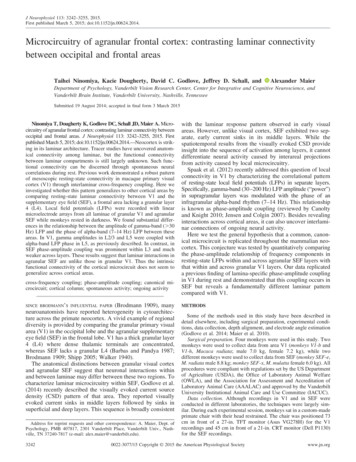
3244FREQUENCY COUPLING IN VISUAL AND AGRANULAR CORTEXAE1ALFig. 1. Laminar electrode placement. A: anatomical MRimage of primary visual cortex (V1) after electroderemoval, revealing penetration tracks. The implantedrecording chamber can be seen extending caudally. B:magnified MRI scan of V1, showing 2 adjacent, parallelelectrode penetration tracks. Note that the MR imagedoes not directly show the cortical lesion but instead thelarger magnetic field distortion (susceptibility artifact)caused by the cerebrospinal fluid that has entered thetrack. C: anatomical MR image of supplementary eyefield (SEF). D: magnified image of region outlined in C.A CT scan of the linear microelectrode array inside therecording chamber (blue line) was coregistered with theMRI. After the boundaries between gray/white matterand gray matter/skull were manually drawn (greenlines), an automated algorithm determined the perpendicular lines along the boundaries (thin yellow lines).Note the perpendicularity of the electrode to the corticalsurface. E: recordings of physiological signals duringelectrode placement. The electrode was advanced 500 m between successive recordings. Note the advancement of the electrocardiogram (red lines) and 1/f neuraldata (blue lines). F: schematic illustration of electrodeconfiguration. Local field potentials (LFPs) were recorded simultaneously across layers of V1 or SEF withthe linear multielectrode array. The location of eachelectrode channel was estimated by the visually evokedcurrent source density (CSD) for each session, whichwas also used to align the data in depth across sessions.Grand average visually evoked CSDs are shown besideNissl sections of V1 and SEF.Celectrode contact a566b66 500 - µV0200 µm100200Time (ms)(nA/mm3)SourceV1: 125SEF: 25Sink-125-251Sexhibiting the highest-magnitude visually evoked current sinks( 450, 0, 750, and 1350 m relative to the location of thehighest-magnitude visually evoked current sink in L3), which provided 1,519, 1,541, 1,678, and 1,392 high alpha segments, respectively, in 621 min of recordings.We extracted periods of high alpha-band power in the bipolar LFPsfor each session. Specifically, bipolar LFPs were band-pass filtered(2-pass least-square finite impulse response filter with an order of 426over 7–14 Hz) and then Hilbert-transformed to acquire the alpha-bandamplitude envelope. Each high alpha segment had an amplitude abovethe 30th percentile of the alpha amplitude distribution within thesession for a minimum time of 800 ms.Alpha-aligned time-frequency representations. TFRs were obtained by aligning time-varying power spectra of the LFP (20 –300Hz) to alpha-band LFP peaks recorded from a single referencechannel (Fig. 2A). More specifically, alpha peaks in the LFP weredefined by identifying zero crossings in the second temporal derivative of the band-limited alpha (7–14 Hz) reference signal. To obtaineach TFR, the spectral power of the bipolar LFP segments aroundalpha peaks was computed with a sliding time window and a singleHanning taper. Power in each frequency band was computed in 1-Hzsteps from 20 to 300 Hz, with a varying window length set to 7 cyclesof the frequency of interest (e.g., the window length for 20 Hz was350 ms, and the window length for 300 Hz was 23.33 ms). Thesealpha-aligned TFRs were averaged and normalized relative to theaverage power per frequency within each channel.To compute statistical significance, randomly shuffled TFRswere obtained by the procedure outlined above but with pairing ofthe LFP for phase extraction from one session with the amplitudefrom a different session recorded in the same area. Results wereJ Neurophysiol doi:10.1152/jn.00624.2014 www.jn.org

FREQUENCY COUPLING IN VISUAL AND AGRANULAR CORTEX3245ABandpassfilteringCalculate power ofSignalampRepeat the procedurewith differentfreq range for Signalampto obtain TFRCalculateaverage poweraround the peakof SignalphFrequencyPowerSignalamp.Example phLowHighPower modulationBBandpassfilteringCalculate amplitudeof Signalamp andphase of SignalphAmplitudeSignalampTime(ms)PhaseCouplingMI 0.01Time(ms)PhaseExample LFP(Coupled)AmplitudeIf not coupledCouplingMI 0-π Phase π-π Phase πTime(ms)SignalphCSignalph (10 Hz)Signalamp (100 Hz)0.2 sHighModulation indexSimulated LFP(Signalph Signalamp Noise)Frequency for amplitude [Hz]Signalamp 100 Hz300100Low1060Frequency for phase [Hz]100200Signalamp 50 Hz6010020 0.20Signalamp 30 HzHigh6020 0.20.2100Power modulationSignalamp 100 HzFrequency (Hz)Frequency (Hz)30000.2Time relative to Signalph peak (s)Averaged signal around Signalph peakJ Neurophysiol doi:10.1152/jn.00624.2014 www.jn.org 0.200.2Low

FREQUENCY COUPLING IN VISUAL AND AGRANULAR CORTEXAV1SEF 1.2 0.4Depth (mm)converted into t-scores, by comparing the alpha-aligned TFRs tothe shuffled TFRs, for cluster-based statistical testing (Maris andOostenveld 2007). We selected four representative channels fromdifferent laminar compartments to assess the relationship betweenthe alpha-band peaks and LFP power within and across the corticallayers. We computed TFRs for the four channels relative to eachalpha reference electrode channel, resulting in 16 TFR combinations for both SEF and V1.Modulation index. The strength of phase-amplitude coupling wasquantified with the MI proposed by Tort et al. (2010) (Fig. 2B). First,the bipolar LFP during periods of high alpha-band power was bandpass filtered into 2-Hz-wide bands centered on the frequency ofinterest, fphase, for all electrode channels. Then the instantaneousphase of a given frequency was estimated by extracting the angle ofthe Hilbert-transformed bipolar band-limited LFP. To analyze theamplitude of the LFP, bipolar LFPs from all electrode channels duringthe high alpha periods (see Data analysis) were band-pass filtered into10-Hz-wide bands, centered on famp. The Hilbert transform wasapplied to these band-limited segments, and the instantaneous amplitude was extracted by taking the absolute value of the output of theHilbert transform. The MI was computed for all pairs of frequencybands, fphase and famp, in 1-Hz steps from 3 to 60 Hz and from 30 to300 Hz, respectively. A matrix of MI values across frequencies forphase versus amplitude was obtained with this procedure. The statistical significance of MI values was assessed with a random permutation test (using 1,000 shuffles) (Spaak et al. 2012). Significant MIvalues were averaged over the alpha (7–14 Hz) and gamma (30 –200Hz) bands to obtain a single MI value for each pair of bipolar LFPs.This yielded a matrix of mean MI values with each element corresponding to a specific combination of cortical depth for alpha phaseand cortical depth for gamma amplitude. The MI matrix of theintersession averages was cubic spline interpolated 10-fold acrossspace. The MI matrices were trimmed after averaging so that eachdata point shown reflects the average over the number of sessionsindicated. Each element of the MI matrix was converted to a t-scoreusing the shuffled MI matrices described above to perform clusterbased statistical testing (Maris and Oostenveld 2007).Validation of TFR and MI analyses. The validity of the TFR andMI analyses was evaluated through analyses of a simulated signal.The simulated signal had three components: Signalph (10-Hz sinewave), Signalamp (100-Hz sine wave with its amplitude coupled withSignalph), and 1/f (pink) noise, with their relative amplitudes set to 5,1, and 105, respectively (Fig. 2C). The TFR computed on the simulated signal showed power around 100 Hz modulating with the phaseof Signalph, verifying the phase-amplitude coupling in the simulatedsignal (Fig. 2C). Similarly, the MI analysis applied to the simulatedsignal produced the highest values between a phase of 10 Hz and anamplitude of 100 Hz (Fig. 2C).Considerable smearing might occur in the lower frequency range ofthe TFRs because the length of the sliding time window is short, e.g.,estimation of power at 30 Hz is based on 2 cycles of alpha. Toclarify whether such an artifact is critical, the TFR analysis wasperformed with Signalamp at low frequencies (30 Hz and 50 Hz; Fig. 0.80 ed powerBNormalized 20406080100Frequency (Hz)Fig. 3. Laminar distributions of LFP power in V1 and SEF. A: average LFPpower as a function of frequency across sessions in V1 (n 15) and SEF (n 16). Red lines mark estimated layer borders. Note the locally increased gammapower in granular V1 compared with the more homogeneous laminar distribution of LFP power in SEF. B: power spectral density of LFP power for mainlaminar compartments (shaded regions indicate SE). Note the overall difference in LFP power between areas as well as the pronounced laminar segregation in SEF. The slight power peak at 60 Hz is due to a line noise artifact.2D). Clear modulation of power was confined around the frequency ofSignalamp, suggesting that smearing is not critical even when the TFRanalysis is applied to the low frequency range.Alpha-aligned current source density analysis. For the alphaaligned CSD analysis, alpha peaks in the unipolar LFP were detectedas described above. LFP segments in a 400-ms window centered onalpha peaks were averaged for each channel. The CSD was calculatedthrough the discrete second spatial derivative as described above. Theaverage CSD around alpha peaks was cubic spline interpolated 10fold across the spatial dimension. This analysis was performed on theelectrode channels described in Alpha-aligned time-frequency representations. The statistical significance of this CSD was assessed withthe procedure applied for alpha-aligned TFRs.RESULTSWe collected laminar LFPs in V1 for 432 min (226 min over11 sessions for monkey V1-b; 206 min over 12 sessions formonkey V1-h) and in SEF for 621 min (339 min over 7 sessionsfor monkey SEF-e; 282 min over 9 sessions for monkey SEF-x).Fig. 2. A: schematic derivation of time-frequency representation (TFR). Example LFP segment is band-pass filtered into 2 frequency ranges of interest foramplitude (Signalamp, red; 20 –300 Hz) and for phase (Signalph, blue; 7–14 Hz). The spectral power of Signalamp is calculated with a sliding time window andtriggered at every peak of Signalph to obtain averaged power of Signalamp around the peak of Signalph. This procedure is repeated for each Signalamp frequencyin 1-Hz steps from 20 to 300 Hz to obtain the full TFR. B: schematic derivation of the modulation index (MI). The first filtering steps are the same as for theTFR. Next, the instantaneous amplitude of Signalamp and the instantaneous phase of Signalph are calculated with the Hilbert transform. The amplitude of Signalampis binned according to the phase of Signalph. The MI is calculated with the algorithm proposed by Tort et al. (2010). The MI equals 0 when the amplitude isdistributed uniformly across the phase cycle (right). C: application of TFR and MI analyses to simulated LFP. Top left: simulated LFP is the sum of 3 spectralcomponents: Signalph (10-Hz sine wave), Signalamp (100-Hz sine wave with amplitude coupled with Signalph), and 1/f (pink) noise. Top right: MI matrix ofsimulated LFP. The procedure shown in B was repeated for Signalph frequencies ranging from 3 to 60 Hz and Signalamp frequencies ranging from 30 to 300 Hz.High MI values occurred around a phase frequency of 10 Hz and amplitude frequency of 100 Hz. Bottom: TFRs of simulated LFP with different frequenciesfor Signalamp (100 Hz, 50 Hz, and 30 Hz from left to right, respectively). Clear modulation of power occurs around each frequency of Signalamp synchronizedwith the peaks and troughs in Signalph (bottom left). Note that the range of the y-axes for the right 2 TFRs is different from that for the left TFR to reveal theentire shape of the modulation. No pronounced smearing can be seen in any TFR.J Neurophysiol doi:10.1152/jn.00624.2014 www.jn.org

FREQUENCY COUPLING IN VISUAL AND AGRANULAR CORTEXPower spectral density differences. We computed the powerspectral density (PSD) of the LFP using the fast Fouriertransform for each of the main laminar compartments of thetwo areas (Fig. 3). As reported previously for V1 (Maier et al.2010), gamma ( 40 Hz) LFP power was higher in L2/3 and L4than in L5 and L6. In contrast, low-frequency ( 10 Hz) LFPpower was higher in deeper than in superficial layers. SEFexhibited a different pattern, with gamma LFP power beinghighest in L3 and also in L5. In summary, the distribution ofpower differed among laminae within each region, and thelaminar pattern of LFP power was qualitatively different between the two areas.The pattern of the laminar PSDs provided another measureto validate laminar depth alignment across sessions (Fig. 4).Data across sessions, each with the array positioned at adifferent depth, were aligned to minimize the difference in thelaminar profile of power in the 40 – 80 Hz range for both V1and SEF. Then the grand average visually evoked CSD wascalculated. The CSD calculated from this alignment procedure(Fig. 4C) was very similar to the CSD calculated from the otheralignment procedure (Fig. 1F). This similarity provides additional converging support for the accuracy of the intersessionalignment applied in this study.Phase-amplitude coupling differences. We next comparedinterlaminar interactions of LFP frequency components in bothareas with cross-frequency analyses (Canolty et al. 2006;Jensen and Colgin 2007; Spaak et al. 2012). We first describeresults showing that V1 and SEF differ in their respectivespectral patterns of interlaminar alpha-gamma coupling. Wethen extend this finding by describing the laminar pattern ofAB3247phase-amplitude coupling across a wider range of frequencies.Finally, we compare the laminar patterns of the alpha-relatedcurrent sinks and sources in V1 and SEF.To confirm the reliability of our data and the validity of ouranalytic approach, we started by evaluating whether our V1data showed a similar laminar profile of alpha-gamma coupling, as reported in a previous study (Spaak et al. 2012). Afteridentifying amplitude peaks in alpha-band (20 –300 Hz) LFPsfrom L5, we computed phase-locked TFRs for LFPs recordedfrom L2/3, L4, L5, and L6. The result can be seen in Fig. 5.TFR colors indicate the relative amount of alpha-locked powermodulation as a function of frequency, while the contoursindicate significant modulations of gamma power based on arandom permutation test (see METHODS for details). In line withSpaak et al. (2012), we found that gamma power in superficiallayers (Fig. 5A) as well as in infragranular L5 (Fig. 5C) wassignificantly coupled to the phase of alpha-band LFPs in L5.Coupling was also observed between gamma power in L4 andL6 and alpha phase in L5, albeit with reduced prominence.Performing the same analysis on the data from SEF, wemade several new observations. First, the overall power modulation in SEF was not as strong as that in V1 (maximum SEFpower modulation around L5 alpha phase was 3% vs. 15%around L5 alpha phase with L2/3 high gamma amplitude inV1). Second, unlike in V1, in L3 of SEF only gamma above 150 Hz coupled with L5 alpha phase (Fig. 5F). Th

cm in front of a 27-in. TFT monitor (Asus VG278H) for the V1 recordings and 45 cm in front of a 21-in. CRT monitor (Dell P1130) for the SEF recordings. Address for reprint requests and other correspondence: A. Maier, Dept. of Psychology, PMB 407817, 2301 Vanderbilt Place, Vanderbilt