WIXLIB

Chapter 1Physical Experiments and ComputerExperiments1.1 IntroductionHistorically, there has been extensive use of both physical experiments and, later,stochastic simulation experiments in order to determine the impact of input variableson outputs of scientific, engineering,or teachnological importance.In the past 15 to 20 years, there has been an increasing use of computer codesto infer the effect of input variables on such outputs. To explain their genesis, suppose that a mathematical theory exists that relates the output of a complex physicalprocess to a set of input variables, e.g., a set of differential equations. Secondly,suppose that a numerical method exists for accurately solving the mathematical system. Typical methods for solving complex mathematical systems include finite element (FE) and computational fluid dynamics (CFD) schemes. In other applications,code output are simply extremely sophisticated simulations run to the point that thesimulation error is essentially zero. Assuming that sufficiently powerful computerhardware and software exists to implement the numerical method, one can treat theoutput of the resulting computer code as an experimental output corresponding theinputs to that code; the result is a computer experiment that produces a “response”corresponding to any given set of input variables.This book describes methods for designing and analyzing research investigationsthat are conducted using computer codes that are used either alone or in addition toa physical experiment.Historically, Statistical Science has been the scientific discipline that createsmethodology for designing empirical research studies and analyzing data fromthem. The process of designing a study to answer a specific research question mustfirst decide which variables are to be observed and the role that each plays, eg, as anexplanatory variable or a response variable. Traditional methods of data collectioninclude retrospective techniques such as cohort studies and the case-control studies used in epidemiology. The gold standard data collection method for establishingcause and effect relationships is the prospective designed experiment. Agriculturalfield experiments were one of the first types of designed experiments. Over time,1

21Physical Experiments and Computer Experimentsmany other subject matter areas and modes of experimentation have been developed. For example, controlled clinical trials are used to compare medical therapiesand stochastic simulation experiments are used extensively in operations research tocompare the performance of (well) understood physical systems having stochasticcomponents such as the flow of material through a job shop.There are critical differences between data generated by a physical experimentand data generated by a computer code that dictate that different methods must beused to analyze the resulting data. Physical experiments measure a stochastic response corresponding to a set of (experimenter-determined) treatment input variables. Unfortunately, most physical experiments also involve nuisance input variables that may or may not be recognized and cause (some of the) variation in theexperimental response. Faced with this reality, statisticians have developed a variety of techniques to increase the validity of treatment comparisons for physicalexperiments. One such method is randomization. Randomizing the order of applying the experimental treatments is done to prevent unrecognized nuisance variablesfrom systematically affecting the response in such a way as to be confounded withtreatment variables. Another technique to increase experimental validity is blocking.Blocking is used when there are recognized nuisance variables, such as different locations or time periods, for which the response is expected to behave differently,even in the absence of treatment variable effects. For example, yields from fieldsin dryer climates can be expected to be different from those in wetter climates andmales may react differently to a certain medical therapy than females. A block isa group of experimental units that have been predetermined to be homogeneous.By applying the treatment in a symmetric way to blocks, comparisons can be madeamong the units that are as similar as possible, except for the treatment of interest.Replication is a third technique for increasing the validity of an experiment. Adequate replication means that an experiment is run on a sufficiently large scale toprevent the unavoidable “measurement” variation in the response from obscuringtreatment differences.In some cases computer experimentation is feasible when physical experimentation is not. For example, the number of input variables may be too large to considerperforming a physical experiment, there may be ethical reasons why a physical experiment cannot be run, or it may simply be economically prohibitive to run an experiment on the scale required to gather sufficient information to answer a particularresearch question. However, we note that when using only computer experiments todetermine the multivariate relationship between a set of inputs and a critical outputbased on an assumed model that has no empirical verification is an extrapolationand all extrapolations can be based on incorrect assumptions.Nevertheless, the number of examples of scientific and technological developments that have been conducted using computer codes are many and growing. Theyhave been used to predict climate and weather, the performance of integrated circuits, the behavior of controlled nuclear fusion devices, the properties of thermalenergy storage devices, and the stresses in prosthetic devices. More detailed motivating examples will be provided in Section 1.2.

1.2Examples3In contrast to classical physical experiments, a computer experiment yields adeterministic answer (at least up to “numerical noise”) for a given set of input conditions; indeed, the code produces identical answers if run twice using the same setof inputs. Thus, using randomization to avoid potential confounding of treatmentvariables with unrecognized “noise” factors is irrelevant–only code inputs can affect the code output. Similarly, blocking the runs into groups that represent “morenearly alike” experimental units is also irrelevant. Indeed, none of the traditionalprinciples of blocking, randomization, and replication are of use in solving the design and analysis problems associated with computer experiments. However, westill use the word “experiment” to describe such a code because the goal in bothphysical and computer experiments is to determine which treatment variables affecta given response and, for those that do, to quantify the details of the input-outputrelationship.In addition to being deterministic, the codes used in some computer experimentscan be time-consuming; in some finite element models, it would not be unusual forcode to run for 12 hours or even considerably longer to produce a single response.Another feature of many computer experiments is that the number of input variablescan be quite large–15 to 20 or more variables. One reason for the large number ofinputs to some codes is that the codes allow the user to not only manipulate thecontrol variables (the inputs that can be set by an engineer or scientist to control theprocess of interest) but also inputs that represent operating conditions and/or inputsthat are part of the physics or biology model being studied but that are known onlyto the agreement of experts in the subject matter field. As examples of the lattertwo types of inputs, consider biomechanics problem of determining the strain thatoccurs at the bone–prosthesis boundary of a prosthetic knee. Of course, prosthesisgeometry is one input that determines the strain. But this output also depends onthe magnitude of the load (an operating condition input) and friction between theprosthetic joint and the bone (a model-based input). Other examples of problemswith both engineering and other types of input variables are given in Section 2.1.This book will discuss methods that can be used to design and analyze computerexperiments that account for their special features. The remainder of this chapterwill provide several motivating examples and an overview of the book.1.2 Examples of Computer ModelsThis section sketches several scientific arenas where computer models are used.Our intent is to show the breadth of application of such models and to providesome feel for the types of inputs and outputs used by these models. The details ofthe mathematical models implemented by the computer code will not be given, butreferences to the source material are provided for interested readers.Example 1.1 (A Physics-based Tower Model). Consider an experiment in which aball is dropped, not thrown, from an initial height x (in meters). The experimentermeasures the time (in seconds) from when the ball is dropped until it hits the ground,

14Physical Experiments and Computer Experimentssay y(x). A computational simulator of this experiment can be derived from Newton’s Law with drag coefficient. Let s(τ) denote the position of the particle at timeτ and let θ denote the coefficient of drag. While the value of θ in the physical experiment is unknown, assume that based on engineering experience, it is possible tospecify a prior distribution, π(θ), of likely values for θ. Then Newton’s law states!ds(τ)d2 s(τ) 1 θ(1.2.1)dτdτ2subject to the initial conditions s(0) x and ds(τ)dτ x 0 0 . The first condition statesthe initial height of the ball is x and the second condition states that the ball isdropped rather than than thrown with some positive initial velocity. The computational model output η(x, θ) is the (smallest) zero of the equations(τ) 0 .(1.2.2)Table 1.1 lists data from a set of computational solutions to this model. The 6670.958η(x, 919Table 1.1 Data from a set of computational simulations of the time for a ball to drop from a givenheight x when the drag coefficient is θ.

1.2Examples5from the computational model is shown in Figure 1.1. Notice that the (x, θ) inputs‘cover’ the input space, that the drop time increases in both x and θ.642000.5x161x40.52000.5θ0100.5θ186Drop TimeDrop Time6426442200.5x100.5θ1024Drop Time6Fig. 1.1 Matrix scatterplot of Tower Data.Corresponding to the computational simulations are the results from six physicalexperiments of timing a dropped ball from a given heightx0.00.20.40.60.81.0Drop Time (sec.)1.59292.17702.87063.83304.59654.7509Table 1.2 Observed times for a ball to drop a given height x.The objectives from this set of experiments might be several fold: (1) to estimate the “true” drag coefficient (or provide a distribution of values consistent withthe data), (2) to predict the Drop Time at an untested height, (3) to quantify theuncertainty in the predicted values in (2).Example 1.2 (Stochastic Evaluation of Prosthetic Devices). see Kevin paper in literature In this example taken from Ong et al (2008), a three-dimensional 14,000-nodefinite element model of the pelvis was used to evaluate the inpact of biomechanicalengineering design variables on the performance of an acetabular cup under a distri-

61Physical Experiments and Computer Experimentsbution of patient loading environments and deviations from ideal surgical insertionparameters.previously developed in detailDesign and environmental variables, their notation, ranges, and distributions 2denotes the chi-square distribution with degrees of freedom; N(2, ?) denotes the normal Gaussian distribution with mean and variance σ2 ; U(a, b) denotes the uniformdistribution over the interval (a, b), DU(a1 , . . . , ad ) denotes the discrete uniform distribution over the values a1 , . . . , ad ; T r(a, b) denotes the triangular distribution over(a, b) centered at a b/2;Example 1.3 (Evolution of Fires in Enclosed Areas). Deterministic computer models are used in many areas of fire protection design including egress (exit) analysis.We describe one of the early “zone computer models” that is used to predict the fireconditions in an enclosed room. Cooper (1980) and Cooper and Stroup (1985) provided a mathematical model and its implementation in FORTRAN for describingthe evolution of a fire in a single room with closed doors and windows that containsan object at some point below the ceiling that has been ignited. The room is assumedto contain a small leak at floor level to prevent the pressure from increasing in theroom. The fire releases both energy and hot combustion by-products. The rate atwhich energy and the by-products are released is allowed to change with time. Theby-products form a plume which rises towards the ceiling. As the plume rises, itdraws in cool air, which decreases the plume’s temperature and increases its volumeflow rate. When the plume reaches the ceiling, it spreads out and forms a hot gaslayer whose lower boundary descends with time. There is a relatively sharp inter-

1.2Examples7face between the hot upper layer and the air in the lower part of the room, which inthis model is considered to be at air temperature. The only interchange between theair in the lower part of the room and the hot upper layer is through the plume. Themodel used by these programs can therefore be described as a two “zone” model.The Cooper and Stroup (1985) code is called ASET (Available Safe EgressTime). Walton (1985) implemented their model in BASIC, calling his computercode ASET-B; he intended his program to be used in the first generation of personalcomputers available at that time of its development. ASET-B is a compact, easy torun program that solves the same differential equations as ASET using a simplernumerical technique.The inputs to ASET-B are the room ceiling height and the room floor area, the height of the burning object (fire source) above the floor, a heat loss fraction for the room (which depends on the insulation in the room,for example), a material-specific heat release rate, and the maximum time for the simulation.The program outputs are the temperature of the hot smoke layer and its distanceabove the fire source as a function of time.Since these early efforts, computer codes have been written to model wildfire evolution as well as fires in confined spaces. As typical examples of thiswork, we point to Lynn (1997) and Cooper (1997), respectively. The publicationsof the Building and Fire Research Laboratory of NIST can be found online athttp://fire.nist.gov/bfrlpubs/. Finally, we mention the review article byBerk et al (2002) which describes statistical approaches for the evaluation of computer models for wildfires. Sahama and Diamond (2001) give a case study usingthe statistical methods introduced in Chapter 3 to analyze a set of 50 observationscomputed from the ASET-B model.To provide a sense of the effect of each of these variables on the evolution ofthe fire, we fixed the heat release rate to correspond to fire material that constitutes a“semi-universal” fire; this heat release profile corresponds to a fire in a “fuel packageconsisting of a polyurethane mattress with sheets and fuels similar to wood cribs andpolyurethane on pallets and commodities in paper cartons stacked on pallets.” (Birk(1997)). Then we varied the remaining four factors using a “Sobol design” (Sobol designs are described in Section ?). We computed the time, to the nearest second,for the fire to reach five feet above the burning fuel package, the fire source.Scatterplots were constructed of each input versus the time required by hot smokelayer to reach five feet above the fire source. Only room area showed strong visualassociations with the output; Figure 1.2 shows this scatterplot (see also Figure 3.10for all four plots). This makes intuitive sense because more by-product is requiredto fill the top of a large room and hence, longer times are required until this layerreaches a point five feet above the fire source. The data from this example will beused later to illustrate several analysis methods.Example 1.4 (Turbulent Mixing). BJW—references?

1Physical Experiments and Computer Experiments503040Time to reach 5 feet (sec.)60708100150200250Room Area (sq. ft.)Fig. 1.2 Scatterplot of room area versus the time for the hot smoke layer to reach five feet abovethe fire source.Example 1.5. “Structural performance is a function of both design and environmental variables. Hip resurfacing design variables include the stem-bone geometry andthe extent of fixation, and environmental variables include variations in bone structure, bone modulus, and joint loading. Environmental variables vary from individual to individual as well as within the same individual over time, and can be treatedstochastically to describe a population of interest.”see paper in literatureExample 1.6 (Qualitative Inputs).Qian, Z., Seepersad, C. C., Joseph, V. R., Allen, J. K., and Wu, C. F. J. (2006),Building Surrogate Models Based on Detailed and Approximate Simulations,ASMEJournal of Mechanical Design, 128, 668–677.Example 1.7 (Formation of Pockets in Sheet Metal). Montgomery and Truss (2001)discussed a computer model that determines the failure depth of symmetric rectangular pockets that are punched in automobile steel sheets; the failure depth is the

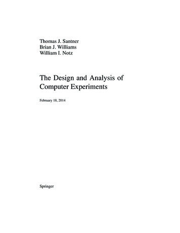
1.2Examples9depth at which the sheet metal tears. Sheet metal, suitably formed in this manner,is used to fabricate many parts of automobiles. This application is but one of manyexamples of computer models used in the automotive industry.Fig. 1.3 Top view of the pocket formed by a punch and die operation. The floor of pocket is theinnermost rectangle. The regions R, s, and r correspond to the similarly labeled regions in the sideview.Fig. 1.4 Side view of part of a symmetric pocket formed by a punch and die operation. The angledside wall is created by the same fillet angle at the top by the die and at the bottom by the edge ofthe punch.

101Physical Experiments and Computer ExperimentsRectangular pockets are formed in sheet metal

The Design and Analysis of Computer Experiments February 18, 2014 Springer. Use the template dedic.tex together with the Springer document class SVMono for monograph-type books or