WIXLIB

CHAPTER 1. PROBABILITY REVIEW3. Sometimes, it is convenient to allow discrete random variables to take the value . Thisis mostly the case when we model the waiting time until the first occurence of an eventwhich may or may not ever happen. If it never happens, we will be waiting forever, andthe waiting time will be . In those cases - when S {1, 2, 3, . . . , } N { } we say that the random variable is extended N-valued. The same applies to the case of N0(instead of N), and we talk about the extended N0 -valued random variables. Sometimes theadjective “extended” is left out, and we talk about N0 -valued random variables, even thoughwe allow them to take the value . This sounds more confusing that it actually is.4. Occasionally, we want our random variables to take values which are not necessarily numbers (think about H and T as the possible outcomes of a coin toss, or the suit of a randomlychosen playing card). Is the collection of all possible values (like {H, T } or { , , , }) iscountable, we still call such random variables discrete. We will see more of that when westart talking about Markov chains.Discrete random variables are very nice due to the following fact: in order to be able to computeany conceivable probability involving a discrete random variable X, it is enough to know howto compute the probabilities P[X x], for all x S. Indeed, if we are interested in figuring outhow much P[X B] is, for some set B R (B [3, 6], or B [ 2, )), we simply pick all x Swhich are also in B and sum their probabilities. In mathematical notation, we haveXP[X B] P[X x].x S BFor this reason, the distribution of any discrete random variable X is usually described via atable x1 x2 x3 . . .,X p1 p2 p3 . . .where the top row lists all the elements of S (the support of X) and the bottom row lists theirprobabilities (pi P[X xi ], i N). When the random variable is N-valued (or N0 -valued), thesituation is even simpler because we know what x1 , x2 , . . . are and we identify the distributionof X with the sequence p1 , p2 , . . . (or p0 , p1 , p2 , . . . in the N0 -valued case), which we call theprobability mass function (pmf) of the random variable X. What about the extended N0 -valuedcase? It is as simple because we can compute the probability P[X ], if we know all theprobabilities pi P[X i], i N0 . Indeed, we use the fact thatP[X 0] P[X 1] · · · P[X ] 1,Pso that P[X ] 1 i 1 pi , where pi P[X i]. In other words,Pif you are given aprobability mass function (p0 , p1 , . . . ), you simply need to compute the sum i 1 pi . If it happensto be equal to 1, you can safely conclude that X never takes the value . Otherwise, theprobability of is positive.The random variables for which S {0, 1} are especially useful. They are called indicators.The name comes from the fact that you should think of such variables as signal lights; if X 1an event of interest has happened, and if X 0 it has not happened. In other words, X indicatesthe occurence of an event. The notation we use is quite suggestive; for example, if Y is theoutcome of a coin-toss, and we want to know whether Heads (H) occurred, we writeX 1{Y H} .Last Updated: December 24, 20106Intro to Stochastic Processes: Lecture Notes

CHAPTER 1. PROBABILITY REVIEWExample 1.2. Suppose that two dice are thrown so that Y1 and Y2 are the numbers obtained (bothY1 and Y2 are discrete random variables with S {1, 2, 3, 4, 5, 6}). If we are interested in theprobability the their sum is at least 9, we proceed as follows. We define the random variable Z the sum of Y1 and Y2 - by Z Y1 Y2 . Another random variable, let us call it X, is defined byX 1{Z 9} , i.e.,(1, Z 9,X 0, Z 9.With such a set-up, X signals whether the event of interest has happened, and we can state ouroriginal problem in terms of X : “Compute P[X 1] !”. Can you compute it?1.4ExpectationFor a discrete random variable X with support , we define the expectation E[X] of X byXE[X] xP[X x],x Pas long as the (possibly) infinite sum x xP[X x] absolutely converges. When the sum doesnot converge, or if it converges only conditionally, we say that the expectation of X is not defined.When the random variable in question is N0 -valued, the expression above simplifies toE[X] Xi pi ,i 0where pi P[X i], for i N0 . Unlike in the general case, the absolute convergence of thedefining series can fail in essentially one way, i.e., whenlimn nXipi .i 0In that case, the expectation does not formally exist. We still write E[X] , but really meanthat the defining sum diverges towards infinity.Once we know what the expectation is, we can easily define several more common terms:Definition 1.3. Let X be a discrete random variable. If the expectation E[X] exists, we say that X is integrable. If E[X 2 ] (i.e., if X 2 is integrable), X is called square-integrable. If E[ X m ] , for some m 0, we say that X has a finite m-th moment. If X has a finite m-th moment, the expectation E[ X E[X] m ] exists and we call it the m-thcentral moment.It can be shown that the expectation E possesses the following properties, where X and Yare both assumed to be integrable:Last Updated: December 24, 20107Intro to Stochastic Processes: Lecture Notes

CHAPTER 1. PROBABILITY REVIEW1. E[αX βY ] αE[X] βE[Y ], for α, β R (linearity of expectation).2. E[X] E[Y ] if P[X Y ] 1 (monotonicity of expectation).Definition 1.4. Let X be a square-integrable random variable. We define the variance Var[X]byVar[X] E[(X m)2 ], where m E[X].pThe square-root Var[X] is called the standard deviation of X.Remark 1.5. Each square-integrable random variable is automatically integrable. Also, if the m-thmoment exists, then all lower moments also exist.We still need to define what happens with random variables that take the value , but thatis very easy. We stipulate that E[X] does not exist, (i.e., E[X] ) as long as P[X ] 0.Simply put, the expectation of a random variable is infinite if there is a positive chance (no matterhow small) that it will take the value .1.5Events and probabilityProbability is usually first explained in terms of the sample space or probability space (whichwe denote by Ω in these notes) and various subsets of Ω which are called events1 Events typicallycontain all elementary events, i.e., elements of the probability space, usually denoted by ω. Forexample, if we are interested in the likelihood of getting an odd number as a sum of outcomesof two dice throws, we build a probability spaceΩ {(1, 1), (1, 2), . . . , (6, 1), (2, 1), (2, 2), . . . , (2, 6), . . . , (6, 1), (6, 2), . . . , (6, 6)}and define the event A which contains of all pairs (k, l) Ω such that k l is an odd number, i.e.,A {(1, 2), (1, 4), (1, 6), (2, 1), (2, 3), . . . , (6, 1), (6, 3), (6, 5)}.One can think of events as very simple random variables. Indeed, if, for an event A, we definethe random variable 1A by(1, A happened,1A 0, A did not happen,we get the indicator random variable mentioned above. Conversely, for any indicator randomvariable X, we define the indicated event A as the set of all elementary events at which X takesthe value 1.What does all this have to do with probability? The analogy goes one step further. If we applythe notion of expectation to the indicator random variable X 1A , we get the probability of A:E[1A ] P[A].Indeed, 1A takes the value 1 on A, and the value 0 on the complement Ac Ω \ A. Therefore,E[1A ] 1 P[A] 0 P[Ac ] P[A].1When Ω is infinite, not all of its subsets can be considered events, due to very strange technical reasons. We willdisregard that fact for the rest of the course. If you feel curious as to why that is the case, google Banach-Tarskiparadox, and try to find a connection.Last Updated: December 24, 20108Intro to Stochastic Processes: Lecture Notes

CHAPTER 1. PROBABILITY REVIEW1.6Dependence and independenceOne of the main differences between random variables and (deterministic or non-random) quantities is that in the former case the whole is more than the sum of its parts. What do I mean bythat? When two random variables, say X and Y , are considered in the same setting, you mustspecify more than just their distributions, if you want to compute probabilities that involve bothof them. Here are two examples.1. We throw two dice, and denote the outcome on the first one by X and the second one byY.2. We throw two dice, and denote the outcome of the first one by X, set Y 6 X and forgetabout the second die.In both cases, both X and Y have the same distributionX, Y 123456161616161616!The pairs (X, Y ) are, however, very different in the two examples. In the first one, if the value ofX is revealed, it will not affect our view of the value of Y . Indeed, the dice are not “connected” inany way (they are independent in the language of probability). In the second case, the knowledgeof X allows us to say what Y is without any doubt - it is 6 X.This example shows that when more than one random variable is considered, one needs toobtain external information about their relationship - not everything can be deduced only bylooking at their distributions (pmfs, or . . . ).One of the most common forms of relationship two random variables can have is the one ofexample (1) above, i.e., no relationship at all. More formally, we say that two (discrete) randomvariables X and Y are independent ifP[X x and Y y] P[X x]P[Y y],for all x and y in the respective supports X and Y of X and Y . The same concept can be appliedto events, and we say that two events A and B are independent ifP[A B] P[A]P[B].The notion of independence is central to probability theory (and this course) because it is relativelyeasy to spot in real life. If there is no physical mechanism that ties two events (like the two dicewe throw), we are inclined to declare them independent2 . One of the most important tasksin probabilistic modelling is the identification of the (small number of) independent randomvariables which serve as building blocks for a big complex system. You will see many examplesof that as we proceed through the course.2Actually, true independence does not exist in reality, save, perhaps a few quantum-theoretic phenomena. Even withapparently independent random variables, dependence can sneak in the most sly of ways. Here is a funny example:a recent survey has found a large correlation between the sale of diapers and the sale of six-packs of beer acrossmany Walmart stores throughout the country. At first these two appear independent, but I am sure you can come upwith many an amusing story why they should, actually, be quite dependent.Last Updated: December 24, 20109Intro to Stochastic Processes: Lecture Notes

CHAPTER 1. PROBABILITY REVIEW1.7Conditional probabilityWhen two random variables are not independent, we still want to know how the knowledge ofthe exact value of one of the affects our guesses about the value of the other. That is what theconditional probability is for. We start with the definition, and we state it for events first: for twoevents A, B such that P[B] 0, the conditional probability P[A B] of A given B is defined as:P[A B] P[A B].P[B]The conditional probability is not defined when P[B] 0 (otherwise, we would be computing- why?). Every statement in the sequel which involves conditional probability will be assumedto hold only when P[B] 0, without explicit mention.The conditional probability calculations often use one of the following two formulas. Bothof them use the familiar concept of partition. If you forgot what it is, here is a definition: acollection A1 , A2 , . . . , An of events is called a partition of Ω if a) A1 A2 . . . An Ω and b)Ai Aj for all pairs i, j 1, . . . , n with i 6 j. So, let A1 , . . . , An be a partition of Ω, and letB be an event.001. The Law of Total Probability.P[B] nXP[B Ai ]P[Ai ].i 12. Bayes formula. For k 1, . . . , n, we haveP[B Ak ]P[Ak ]P[Ak B] Pn.i 1 P[B Ai ]P[Ai ]Even though the formulas above are stated for finite partitions, they remain true when the numberof Ak ’s is countably infinite. The finite sums have to be replaced by infinite series, however.Random variables can be substituted for events in the definition of conditional probability asfollows: for two random variables X and Y , the conditional probabilty that X x, given Y y(with x and y in respective supports X and Y ) is given byP[X x Y y] P[X x and Y y].P[Y y]The formula above produces a different probability distribution for each y. This is called theconditional distribution of X, given Y y. We give a simple example to illustrate this concept.Let X be the number of heads obtained when two coins are thrown, and let Y be the indicatorof the event that the second coin shows heads. The distribution of X is Binomial:!012X 1,11424or, in the more compact notation which we use when the support is clear from the contextX ( 14 , 12 , 14 ). The random variable Y has the Bernoulli distribution Y ( 21 , 12 ). What happensLast Updated: December 24, 201010Intro to Stochastic Processes: Lecture Notes

CHAPTER 1. PROBABILITY REVIEWto the distribution of X, when we are told that Y 0, i.e., that the second coin shows heads. Inthat case we have P[X 0,Y 0]P[ the pattern is TT ]1 1/4x 0 P[Y 0] P[Y 0]1/2 2 , 0]is HT ]1/4P[X x Y 0] P[X 1,Y P[ the pattern 1/2 12 ,x 1P[Y 0]P[Y 0] P[X 2,Y 0]P[ well, there is no such pattern ]0 1/2 0 , x 2P[Y 0]P[Y 0]Thus, the conditional distribution of X, given Y 0, is ( 21 , 12 , 0). A similar calculation can be usedto get the conditional distribution of X, but now given that Y 1, is (0, 12 , 21 ). The moral of thestory is that the additional information contained in Y can alter our views about the unknownvalue of X using the concept of conditional probability. One final remark about the relationshipbetween independence and conditional probability: suppose that the random variables X and Yare independent. Then the knowledge of Y should not affect how we think about X; indeed, thenP[X x Y y] P[X x, Y y]P[X x]P[Y y] P[X x].P[Y y]P[Y y]The conditional distribution does not depend on y, and coincides with the unconditional one.The notion of independence for two random variables can easily be generalized to largercollectionsDefinition 1.6. Random variables X1 , X2 , . . . , Xn are said to be independent ifP[X1 x1 , X2 x2 , . . . Xn xn ] P[X1 x1 ]P[X2 x2 ] . . . P[Xn xn ]for all x1 , x2 , . . . , xn .An infinite collection of random variables is said to be independent if all of its finite subcollections are independent.Independence is often used in the following way:Proposition 1.7. Let X1 , . . . , Xn be independent random variables. Then1. g1 (X1 ), . . . , gn (Xn ) are also independent for (practically) all functions g1 , . . . , gn ,2. if X1 , . . . , Xn are integrable then the product X1 . . . Xn is integrable andE[X1 . . . Xn ] E[X1 ] . . . E[Xn ], and3. if X1 , . . . , Xn are square-integrable, thenVar[X1 · · · Xn ] Var[X1 ] · · · Var[Xn ].EquivalentlyCov[Xi , Xj ] E[(X1 E[X1 ])(X2 E[X2 ])] 0,for all i 6 j {1, 2, . . . , n}.Remark 1.8. The last statement says that independent random variables are uncorrelated. Theconverse is not true. There are uncorrelated random variables which are not independent.Last Updated: December 24, 201011Intro to Stochastic Processes: Lecture Notes

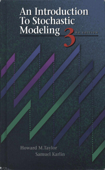
CHAPTER 1. PROBABILITY REVIEWWhen several random variables (X1 , X2 , . . . Xn ) are considered in the same setting, we often group them together into a random vector. The distribution of the random vector X (X1 , . . . , Xn ) is the collection of all probabilities of the formP[X1 x1 , X2 x2 , . . . , Xn xn ],when x1 , x2 , . . . , xn range through all numbers in the appropriate supports. Unlike in the caseof a single random variable, writing down the distributions of random vectors in tables is a bitmore difficult. In the two-dimensional case, one would need an entire matrix, and in the higherdimensions some sort of a hologram would be the only hope.The distributions of the components X1 , . . . , Xn of the random vector X are called themarginal distributions of the random variables X1 , . . . , Xn . When we want to stress the fact thatthe random variables X1 , . . . , Xn are a part of the same random vector, we call the distributionof X the joint distribution of X1 , . . . , Xn . It is important to note that, unless random variablesX1 , . . . , Xn are a priori known to be independent, the joint distribution holds more informationabout X than all marginal distributions together.1.8ExamplesHere is a short list of some of the most important discrete random variables. You will learn aboutgenerating functions soon.Example 1.9.Bernoulli. Success (1) of failure (0) with probability p (if success is encoded by 1, failure by 1 and p 12 , we call it the coin toss).0.70.60.50.40.30.20.10.0-0.50.00.5Last Updated: December 24, 20101.0.parameters : p (0, 1) (q 1 p).notation : b(p).support : {0, 1}.pmf : p0 p and p1 q 1 p.generating function : ps q.mean : p .standard deviation :pq.figure :the mass function a Bernoulli distribution with p 1/3.Binomial. The number of successes in n repeti-12Intro to Stochastic Processes: Lecture Notes

CHAPTER 1. PROBABILITY REVIEWtions of a Bernoulli trial with success arameters : n N, p (0, 1) (q 1 p).notation : b(n, p).support : {0, 1, . . . , n}.pmf : pk nk pk q n k , k 0, . . . , n.generating function : (ps q)n.mean : np .standard deviation :npq.figure :mass functions of three binomial distributions with n 50 and p 0.05 (blue), p 0.5(purple) and p 0.8 (yellow).Poisson. The number of spelling mistakes one makes while typing a single page.0.40.30.20.10510152025.parameters : λ 0.notation : p(n, p).support : N0k.pmf : pk e λ λk! , k N0.generating function : eλ(s 1).mean : λ .standard deviation :λ.figure : mass functions of two Poisson distributions with parameters λ 0.9 (blue) and λ 10(purple).Geometric. The number of repetitions of a Bernoulli trial with parameter p until the firstsuccess.0.30.parameters : p (0, 1), q 1 p.notation: g(p)0.25.support : N00.20.pmf : pk pq k 1 , k N0p.generating function : 1 qs0.15.mean : pq 0.100.050510152025Last Updated: December 24, 201030q.standard deviation : p.figure : mass functions of two Geometric distributions with parameters p 0.1 (blue) and p 0.4(purple).13Intro to Stochastic Processes: Lecture Notes

CHAPTER 1. PROBABILITY REVIEWNegative Binomial. The number of failures it takes to obtain r successes in repeated independent Bernoulli trials with success probability p.parameters : r N, p (0, 1) (q 1 p).notation : g(n, p).support : N0 r k N0.pmf : pk

Introduction to Stochastic Processes - Lecture Notes (with 33 illustrations) Gordan Žitković De