Transcription
RSFT: A Realistic High Dimensional SparseFourier Transform and Its Application in RadarSignal ProcessingShaogang Wang, Vishal M. Patel and Athina PetropuluDepartment of Electrical and Computer EngineeringRutgers University94 Brett Road, Piscataway, NJ 08854Email: {shaogang.wang, vishal.m.patel, athinap}@rutgers.eduestimates. However, the computation of gradient descent isnot efficient, due to the unknown gradient of the signal in thefrequency domain. An SFT algorithm for off-grid frequencieswas proposed by Boufounos et al. in [10]. The underlyingassumption in [10] is that signal and noise are well separatedby predefined gaps in the frequency domain. However, thisassumption does not hold for many practical signal processingapplications.In this paper, we propose a new algorithm called RealisticSparse Fourier Transform (RSFT), which does not requires thefrequencies to be on-grid and does not rely on the restrictiveassumption that signal and noise are well separated by predefined gaps in the Fourier domain. Furthermore, we extend theproposed algorithm to arbitrary fixed high dimensions so thatit can be used to replace the N -dimensional FFT (N-D FFT)in a sparse setting. To the best of our knowledge, the RSFTalgorithm is the first SFT algorithm, which addresses the issueof off-grid frequencies for arbitrary high dimensional signals.Finally, we present an application of the RSFT algorithm inmulti-dimensional radar signal processing, in which a 3-DRSFT is applied on short range ubiquitous radar [11] (SRUR)to detect targets and estimate their range, velocity and directionof arrival (DOA). Due to the computational efficiency of RSFT,a faster reaction or lower cost of hardware for this kind of radaris expected.Notation: We use lower-case and upper-case bold letters todenote vectors and matrices, respectively. [S] refers to the setof indices {0, · · · , S 1}. The DFT of signal s is denoted asŝ.This paper is organized as follows. A brief backgroundon the SFT algorithm is given in Section II. Details ofthe proposed RSFT algorithm are given in Section III. Anapplication of the RSFT algorithm in radar signal processingis presented in Section IV. Section V concludes the paper witha brief summary and discussion.Abstract—We propose a realistic high dimensional sparseFourier transform (RSFT) algorithm, which detects frequenciesin multidimensional data, provided that the data is sparse in thefrequency domain. Although sparsity has been exploited before toreduce the complexity of the Discrete Fourier Transform, unlikeprevious approaches, the RSFT allows for off-grid frequencies.We provide a concrete application example on short rangeubiquitous radar signal processing, and verify the feasibility ofthe RSFT in that scenario via simulations.Index Terms—Array signal processing, sparse Fourier transform, radar signal processing.I. I NTRODUCTIONMany practical applications in radar, communications andimaging require one to take the Discrete Fourier Transform(DFT) of high-dimensional signals in order to identify frequencies in the data. The DFT is usually implemented via the FastFourier Transform (FFT), whose computational complexityis O(N log N ) for N data points. Recently, by leveragingthe sparsity of signals in the frequency domain, the SparseFourier Transform (SFT) [1], [2] can further reduce thecomplexity required to identify the underlying frequencies.Different versions of the SFT related techniques have beensuccessfully applied in several practical applications, such asa fast Global Positioning System (GPS) receiver, wide-bandspectrum sensing, light field reconstruction, etc. [3]–[5].High order extension of the SFT has also been considered.Andre et al. [6] extended the exactly-K-sparse SFT algorithmfrom [1] into two dimensions. Ghazi et al. [7] proposed asample optimal 2-D SFT both for exactly sparse and approximately sparse signals. Ong et al. [8] proposed a 2-D SFTalgorithm based on sparse-graph decoding. An extension to anarbitrary constant dimension is reported in [9]. However, allthe aforementioned algorithms rely on a grid, and assume thatthe signal frequencies are on the grid. In practice, however, thesignal frequencies lie in the continuous space of [0, 2π), andare usually off-grid. The consequence of off-grid frequenciesis leakage to other frequency bins, which essentially destroysthe sparsity of the signal. To refine the estimation of off-gridfrequencies, in [5], Shi et al. proposed a gradient descentbased method to find off-grid frequencies from the initial SFTII. BACKGROUNDAs opposed to the FFT that computes the coefficients ofall N frequency components of a N -samples long signal, the1
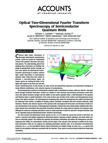
SFT [2] computes only the K frequency components of a Ksparse signals. At a high level, the SFT consists of two kindsof loops, i.e., the Location loop and the Estimation loop. Theformer finds the indices of the K most significant frequenciesin the input signal, while the latter estimates the correspondingFourier coefficients. Here we emphasize on Location morethan Estimation, since the former is more relevant to theradar application that we consider. The Location step providesfrequency locations, which in the radar case is directly relatedto target parameters.In the Location loop, a permutation procedure reorders theinput data in the time domain, causing the frequencies to alsoreorder. The permutation causes closely spaced frequenciesto appear in well separated locations with high probability.Mathematically, the permutation is defined as(1)where xi is the ith entry of input signal x CN , σ, τ [N ],and σ is invertible mod N , i.e., there exists a σ 1 satisfyingσσ 1 1 (mod N ). Consequently, the frequency is dilatedmodularly by σ times, and an additional phased rotation by τ jτ 2π\N . It is also assumedis introduced, i.e., (Pσ,τ x)σi x̂i ethat the data length for each dimension is a power of 2. Then,a flat-window [2] is applied on the permuted signal for thepurpose of extending a single frequency into a (nearly) boxcar,for a reason that will become apparent in the following. Thewindowed data are aliased, by creating a periodic extension ofthe data with period B with B N , and B a power of 2. Thefrequency domain equivalent of this aliasing is undersamplingby N/B. The window used at the previous step ensures thatno peaks are lost due to the effective undersampling in thefrequency domain. After this stage, a FFT of length B of oneperiod is employed.The first detection stage finds the significant frequencies’peaks and their indices are reverse mapped into the originalfrequency space. However, the reverse mapping yields notonly the true location of the signal frequency, but also N/Bambiguous locations for each significant frequency. To removethe ambiguity, multiple iterations of Location with randomizedpermutation are performed. Finally, the second stage detectionlocates the K most significant frequencies from the accumulated data for each iteration.608040Amplitude / dBAmplitude / dB6040200200-200246-40802Frequency / rad(a)868604060Amplitude / dB6(b)80402004Frequency / radAmplitude / dB(Pσ,τ x)i xσi τ ,frequency component would easily mask the main lobe of aweak frequency component (See Fig. 1 (c)). To address thisproblem, we multiply the received time domain signal witha window before permutation, and call this procedure Prepermutation Windowing. The idea is to confine the leakagewithin a finite number of frequency bins, as illustrated in Fig.1.The choice of the pre-permutation window is determinedby dynamic range, frequency resolution and computationalcomplexity requirements. More specifically, the dynamic rangespecification determines the attenuation of the side-lobes, andthe side-lobe level should be lower than the noise level afterwindowing. However, the larger attenuation of the side-lobes,the more wide would be the main-lobe, leading to a worsenresolution in frequency domain. Meanwhile, a more broadenmain-lobe will cause greater computational overhead, whichwill be discussed in Section III-D.200-2002468-40Frequency / rad024Frequency / rad(c)(d)Fig. 1. Effect of pre-permutation Windowing. The signal contains twosignificant frequency components, one of which is 15dB stronger than theother. A Dolph-Chebyshev window is applied to the time-domain signal.Windowed signal after permutation is more sparse in the frequency domain ascompared to the permuted unwindowed signal. (a) Spectrum of unwindowedsignal. (b) Spectrum of windowed signal. (c) Spectrum of unwindowed signalafter permutation. (d) Spectrum of windowed signal after permutation.III. T HE RSFT A LGORITHMB. High Dimensional ExtensionsIn this section, we introduce the proposed RSFT algorithm,which is basically an SFT that is robust to off-grid frequenciesand present its extensions to high dimensional problems.Due to the separability of the DFT, one could easily extendthe FFT to high dimensions by simply applying 1-D FFTon each dimension of the data sequentially. For the SFTalgorithm, however, the extension is not obvious. In whatfollows, we elaborate on the high dimensional extension forits main stages.1) Windowing: In the pre-permutation windowing and theflat-windowing stages, the window for each dimension isdesigned separately. After that, the high dimension widow isgenerated by combining each 1-D window. For instance, inthe 2-D case, assuming that wx and wy are the two windowsA. Leakage Suppression for Off-grid FrequenciesThe SFT algorithm only holds for the discrete on-gridfrequencies. In real world applications, the frequencies arecontinuous and can take any value in [0, 2π). When fittinga grid on these frequencies, leakage occurs from off-gridfrequencies, which can jeopardize the natural sparsity of thesignal. As a result, it is difficult to determine the frequencydomain peaks after permutation, since the leakage of a strong2
in the x and y dimension, respectively, a 2D window can becomputed asWxy wx wyH ,(2)space. The combination of the reverse mapped indices fromeach dimension provides the tentative locations of the originalfrequency components. Assuming the side-lobes are below thenoise level after pre-permutation windowing, empirically, wecan choose d asYd round(di ),(3)where (·)H denotes for the conjugate transpose. Fig. 2 shows acompound 2-D window which is a combination of a hammingwindow and a Dolph-Chebyshev window. We apply thosewindows on the data by point-wise multiplications.i [U ]where U is the number of dimensions, round(·) denotes forrounding to the nearest integer, and di is the 6.0-dB bandwidthof the pre-permutation window for the ith dimension. Forinstance, according to [12], a Hamming window has its 6.0-dBbandwidth approximately as 1.81. As a result, a 2-D Hammingwindow gives d 3.5) Accumulation and second stage detection: The accumulation stage collects the tentative frequency locations foundin the reverse mapping for each iteration, and the number ofoccurrences for each location is calculated after running overT iterations. The second stage detection finds K peaks in thedata with the highest number of 40.20020040060080010001200(a)(b)Fig. 2. Compound Window in 2-D. (a) Top: a 64-points Hamming window;bottom: a 1024-points Dolph-Chebyshev window. (b) The 2D window.2) Permutation: The permutation parameters are generatedfor each dimension in a random way according to (1). Then,we carry the permutation on each dimension sequentially. Anexample for the 2-D case is illustrated in Fig. 12629322730yx25Based on the discussion above, we summarize the RSFTmethod in Algorithm 1. We set τ 0 in each permutation,since the random phase rotation does not affect the performance of a detector after taking magnitude of the signal inthe intermediate stage.Algorithm 1 RSFT algorithmInput: complex signal r in any fixed high dimensionOutput: o, sparse frequency locations of input signal1: procedure RSFT(r)2:Pre-Permutation Windowing: y Wr3:Generate a set of σ randomly for each dimension4:x 05:for i 0 to T do6:Permutation: p Pσ y7:Flat-windowing: z Wf p8:Aliasing: a Aliasing(z)9:N-D FFT: â FFT(a)10:First-stage-detection: c Det1( â 2 )11:Reverse-mapping: xi Reverse(c)12:Accumulation: x x xi13:end for14:Second-stage-detection: o Det2(x)15:return o16: end procedurex(a)yC. The RSFT 22912151013161114xy1 5 17 214 8 20 247 3 23 192 6 18 2225 29 9 1328 32 12 1631 27 15 1126 30 10 14x(c)(d)Fig. 3. Permutation and Aliasing in 2D. (a) Original 2D data forms a 4 8matrix. (b) Permutation in x dimension, σx 3, τx 0. (c) Permutation iny dimension, σy 3, τy 0. After permutation, data is divided into four2 4 sub-matrices. (d) Aliasing by adding sub-matrices from (c).3) Aliasing: The aliasing stage compresses the high dimensional data into much smaller size. In 2-D, as shown in Fig.3 (d), a periodic extension of the Nx Ny data matrix iscreated with period Bx in the x dimension and By in the ydimension, with Bx Nx and By Ny , and the basicperiod is extracted.4) First stage detection and reverse mapping: We carryfirst stage detection after taking the magnitude of N-D FFTon the aliased data. Since the size of aliased data is muchsmaller than original size, the saving of the computationis remarkable. After that, we find the dK, d 1 highestpeaks and then reverse map their indices back to the originalD. Computational ComplexityWe compute the computational complexity of the RSFTalgorithm by counting the number of operations in Algorithm1, as shown in Table I. The RSFT yields a complexity of KdNO T (N B B log B ) N ,(4)B3
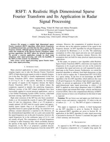
while the N-D FFT gives the complexity of O(N log N ). HereN, B denote for the total number of data points in the originaland shrunken high dimensional dataset, respectively. From Fig.4, one can see that the complexity ratio of FFT over RSFTrises almost linearly versus N , which grows exponentially.For N 250 , B 212 , T 5, K 100, d 2,the RSFT algorithm is approximately 8 times more efficientthan the FFT. Note that the core operation in RSFT is stillFFT but on a reduced dimensional space. By leveraging theexisting high performance FFT libraries such as FFTW [13],the implementation of the RSFT algorithm could be furtherimproved.As discussed in Section III-A, the choice of pre-permutationwindow is a compromise between the resolution and dynamicrange specifications. Now, from Eq. (3) and (4), we can seethe pre-permutation window also affects the complexity ofthe RSFT, i.e., a window with larger d will demand morecomputation, as shown in Fig. 4.The complexity of RSFT is also influenced by B. Withother parameters fixed, we can solve the optimal B, whichminimizes f in Eq. (4). In the high dimensional setting, Bis the multiplication Qof the shrunken data length in eachdimension, i.e., B i [U ] Bi , with Bi a power of 2. Andin order to hash each significant frequency into a distinctlocation of the shrunken space with high probability, we makeB dK.TABLE IC OMPUTATIONAL C OMPLEXITY OF RSFTProcedurePre-Permutation WinPermutationFlat WinAliasingFFTSquareFirst Stage DetectionReverse MappingSecond stage DetectionTotal OperationsComplexityNumber of OperationsNTNTNT B(N/B 1)TBlog B2TBTBT KdN/BNT (3N B BlogB KdN) 2N 2B) NO T (N B B log B KdNBWhile many applications satisfy these requirements, in whatfollows, we discuss an example in SRUR signal processing.A. Short Range Ubiquitous Radar (SRUR)An ubiquitous radar [11] or SIMO radar can see targetseverywhere at anytime without steering its beams as a traditional phased array radar does. In SRUR, a broad transmittingbeam patten is achieved by an omnidirectional transmitterand multiple narrow beams are formed simultaneously afterreceiving of the reflected signal. The beam pattens of anubiquitous radar is shown in Fig. 5 with an Uniform LinearArray (ULA) configuration.Ratio of Complexity, FFT / RSFT98Tx BeamRx Beam76543K 10, d 2K 100, d 2K 100, d 4021106108101010121014TxAD1016DDSNFig. 4. Complexity Ratio, FFT over RSFT. B 212 , T 5.ADADDSPIV. RSFT FOR U BIQUITOUS R ADAR S IGNAL P ROCESSINGFig. 5. Ubiquitous Radar System Structure and Transmitting / ReceivingBeam Patten. A broad beam patten is transmitted with an omnidirectionalantenna, while multiple narrow beams are formed simultaneously by thereceiving array. Each receiving channel is mixed with a coupled signal fromthe transmitter to de-chirp the LFMCW signal, before the A/D converting.The complexity analysis above reveals that the RSFT algorithm can greatly reduce the complexity of certain high dimensional problems. This can be signifiant in many applications,since lower complexity means faster reaction time and moreeconomical hardware. However, in order to apply RSFT, thesignal to be processed should meet the following requirements: It should be sparse in some domain. It should be sampled uniformly whether in temporal orspacial domain. The SNR should be moderately high so that the algorithmcan detect the peaks of significant frequencies reliably.An SRUR with range coverage of several kilometers couldbe important both in military and civilian vehicular applications. For instance, in an active protection system [14], sensorson the protected vehicle have to detect and locate the warheadsfrom a closely fired rocket-propelled grenade (RPG) withinmilliseconds. Among other sensors, SRUR’s simultaneouswide angle coverage, high precision of measurement and allweather operation make it the ideal sensor for such situation.In order to achieve high range resolution and cover nearrange, SRUR utilizes a LFMCW waveform, as shown in Fig.4
fTransmitingReceivingRangeBwR 3DFFT . 7. Conventional Processing Scheme for SRUR.tFig. 6. LFMCW Waveform. The signal frequency change linearly in timewith a repetition internal Tp . A burst contains M repetitions. The range offrequency changing is the bandwidth of the system. The received signal is adelayed version of the transmitted signal.Loop for T AliasingM 3DFFT 2VDOA(6)which is a superposition of K sinusoids and additive noisen(t). For the kth sinusoid, a[k] represents its amplitude and[k][k]fr , fd are the frequency components respect to target’srange and velocity respectively, i.e.,[k]2v t ,λ1st DetectionC. Simulations[k][k]fdReverseMappingAlthough the number of samples of SRUR is reducedsignificantly with the analog de-chirp processing, the realtimeprocessing with 3-D FFT is still challenging. The RSFT algorithm is suitable for reducing the computational complexity ofSRUR since, 1) the number of targets is usually much smallerthan the number of spatial resolutions cells, which impliesthat the signal is sparse after proper translation; 2) with anULA and digitization of each received element, the signal isuniformly sampled both in spatial and temporal domain; and3) the short range coverage implies that moderate high SNRis easy to achieve.The RSFT-based SRUR processing architecture is shownin Fig. 8. Compared to the conventional processing, the 3-DFFT is replaced with the looping block, in which the aliasingprocedure converts the data cube dimension from R N Mto B C D. The 3-D FFT operated on the smaller datacube could save the computation time significantly.k [K][k]Acc forTiterationsB. RSFT-based SRUR Signal Processing n(t),2αrt, c2ndDetectionFig. 8. RSFT Based Processing Scheme for SRUR.(5)where Tp is the repetition interval (RI), v [M ] denotes thevth RI, A is amplitude of the signal, fc is the carrier frequencyand α is the chirp rate. Furthermore, without loss of generality,we assume that the initial phase of the signal is zero.Upon reception, a de-chirp process is implemented by mixing the received signal with the transmitted signal, followedby a lowpass filter. The received signal is a delayed versionof the transmitted one, hence by mixing the two signals, therange information of the targets is linearly encoded in thedifference of the frequencies. Hence for the ith , i [N ]receiving channel, the de-chirped signal is expressed as X[k]ri a[k] cos 2π((fr[k] fd )(t vTp ) iπ sin θ[k]fr[k]Digitals(t, v) A cos(2π(fc (t vTp ) πα(t vTp )2 ),Analog6. Mathematically, the transmitted waveform can be expressedasIn this section, we verify the feasibility of RSFT-basedSRUR processing and compare to the SFT-based processingvia simulations. The main parameters of the system are listedin Table II. The design of the system can guarantee nonambiguous measurements of the target’s range and velocity,assuming the maximum range and velocity are less than 1.5kmand 300m/s, respectively.We generate a signal from 4 targets according to (6). Theparameters of targets can be arbitrarily chosen within the unambiguous space, which implies the corresponding frequencycomponents do not necessarily lie on the grid points. Thetargets’ parameters used in the simulation are listed in TableIII.The SFT from [2] is 1-dimensional. In order to reconstructtargets in the 3-D space, we extend the SFT to high dimensionwith the techniques described in Section III-B. In the experiment, we choose B, C, D equal to 64, 32, 16, respectively, andgradually increase the number of counting peaks in the first(7)[k]where rt , vt , c are the kth target’s range, velocity and speedof wave propagation respectively.The DOA of the kth target, i.e., θ[k] is defined as theangle between the line of sight (from the array center tothe target) and the array normal. Assuming that the elementwise spacing is λ/2, under the narrowband signal assumption,θ[k] will cause an increase of phase at the neighboring arrayelement equal to π sin θ[k] . We omit the constant phase termin each sinusoids of Eq. (6), since they are irrelevant to theperformance of the algorithm.After AD conversion of each receiving channel, we can usethe processing scheme shown in Fig. 7 to detect the targetsas well as estimate their range, velocity and DOA. More[k][k]specifically, grid-based versions of fr , fd , π sin θ[k] can becalculated by applying a 3-D FFT on the windowed data cube,followed by a detection procedure.5
Further work is needed to determine the ability of RSFT todetect weak targets, and its behavior when the exact sparsityis not known.TABLE IISRUR PARAMETERSParameterNumber of range binsNumber of receiving elementsNumber of RIWave lengthWave propagation speedBandwidthRepetition intervalMaxima rangeChirp rateSampling frequency (IQ)SymbolRNMλcBwTpRmaxαfsValue204864320.03m3 108 m/s150M Hz5 10 5 s1.5 103 m3 1012 Hz/s41M HzACKNOWLEDGEMENTThe authors would like to thank Dr. Predrag Spasojevic andDr. Anand Sarwate from Rutgers university for initial supportof this work. The work of SW was jointly supported by ChinaScholarship Council and Shanghai Institute of SpaceflightElectronics Technology. The work of VMP was partiallysupported by an ARO grant W911NF-16-1-0126.R EFERENCESTABLE IIITARGET PARAMETERSTarget1234Range (m)1000500350350Velocity (m/s)10050240240DOA ( )300 16 20[1] H. Hassanieh, P. Indyk, D. Katabi, and E. Price, “Nearly optimalsparse fourier transform,” in Proceedings of the forty-fourth annual ACMsymposium on Theory of computing, pp. 563–578, ACM, 2012.[2] H. Hassanieh, P. Indyk, D. Katabi, and E. Price, “Simple and practicalalgorithm for sparse fourier transform,” in Proceedings of the Twentythird Annual ACM-SIAM Symposium on Discrete Algorithms, SODA’12, pp. 1183–1194, SIAM, 2012.[3] H. Hassanieh, F. Adib, D. Katabi, and P. Indyk, “Faster gps via the sparsefourier transform,” in Proceedings of the 18th annual internationalconference on Mobile computing and networking, pp. 353–364, ACM,2012.[4] H. Hassanieh, L. Shi, O. Abari, E. Hamed, and D. Katabi, “Ghz-widesensing and decoding using the sparse fourier transform,” in INFOCOM,2014 Proceedings IEEE, pp. 2256–2264, IEEE, 2014.[5] L. Shi, H. Hassanieh, A. Davis, D. Katabi, and F. Durand, “Light fieldreconstruction using sparsity in the continuous fourier domain,” ACMTransactions on Graphics (TOG), vol. 34, no. 1, p. 12, 2014.[6] A. Rauh and G. R. Arce, “Sparse 2d fast fourier transform,” Proceedingsof the 10th International Conference on Sampling Theory and Applications, 2013.[7] B. Ghazi, H. Hassanieh, P. Indyk, D. Katabi, E. Price, and L. Shi,“Sample-optimal average-case sparse fourier transform in two dimensions,” in Communication, Control, and Computing (Allerton), 2013 51stAnnual Allerton Conference on, pp. 1258–1265, IEEE, 2013.[8] F. Ong, S. Pawar, and K. Ramchandran, “Fast and efficient sparse 2ddiscrete fourier transform using sparse-graph codes,” arXiv preprintarXiv:1509.05849, 2015.[9] P. Indyk and M. Kapralov, “Sample-optimal fourier sampling in anyconstant dimension,” in Foundations of Computer Science (FOCS), 2014IEEE 55th Annual Symposium on, pp. 514–523, IEEE, 2014.[10] P. Boufounos, V. Cevher, A. C. Gilbert, Y. Li, and M. J. Strauss, “What’sthe frequency, kenneth?: Sublinear fourier sampling off the grid,” inApproximation, Randomization, and Combinatorial Optimization. Algorithms and Techniques, pp. 61–72, Springer, 2012.[11] M. Skolnik, “Systems aspects of digital beam forming ubiquitous radar,”tech. rep., DTIC Document, 2002.[12] F. J. Harris, “On the use of windows for harmonic analysis with thediscrete fourier transform,” Proceedings of the IEEE, vol. 66, no. 1,pp. 51–83, 1978.[13] M. Frigo and S. G. Johnson, “Fftw: An adaptive software architecture forthe fft,” in Acoustics, Speech and Signal Processing, 1998. Proceedingsof the 1998 IEEE International Conference on, vol. 3, pp. 1381–1384,IEEE, 1998.[14] D. A. Schade, T. C. Winant, J. Alforque, J. Faul, K. B. Groves,V. Horvatich, M. A. Middione, C. Tarantino, and J. R. Turner, “Fastacting active protection system,” Apr. 10 2007. US Patent 7,202,809.SNR (dB)0 10 20 20Fig. 9. Target Reconstruction via 3-D SFT and RSFT. The SFT-basedprocessing recovers the side-lobes of the stronger targets, while the RSFTbased method only recovers the main-lobes of targets.stage detection until all the targets are recovered. Fig. 9 showsthe targets reconstruction results from both methods. The SFTbased method shows the side-lobes of the stronger targets,while the RSFT-based method only recovers the (extended)main-lobes of all the targets.V. D ISCUSSION AND C ONCLUSIONIn this paper, we have addressed some practical limitationsof the SFT algorithm by developing the RSFT algorithm. Ithas been shown that the RSFT algorithm is computationallymore efficient than N-D FFT in sparse settings and is robustto off-grid frequencies. Furthermore, we have presented anapplication of our RSFT algorithm in ubiquitous radar signalprocessing.6
Abstract—We propose a realistic high dimensional sparse Fourier transform (RSFT) algorithm, which detects frequencies in multidimensional data, provided that the data is sparse in the frequency domain. Although sparsity has been exploited before to reduce the complexity o