Transcription
Six Sigma Quality: Concepts & Cases Volume ISTATISTICAL TOOLS IN SIX SIGMA DMAIC PROCESS WITHMINITAB APPLICATIONSChapter 6PROCESS CAPABILITY ANALYSIS FORSIX SIGMA 2010-12 Amar Sahay, Ph.D.1
Chapter 6: Process Capability Analysis for Six SigmaCHAPTER OUTLINEProcess CapabilityProcess Capability AnalysisDetermining Process CapabilityImportant Terms and Their DefinitionsShort‐term and Long‐term VariationsProcess Capability Using HistogramsProcess Capability Using Probability PlotEstimating Percentage Nonconforming for Non‐normal Data: Example 1Estimating Nonconformance Rate for Non‐normal Data : Example 2Capability Indexes for Normally Distributed Process DataDetermining Process Capability Using Normal DistributionFormulas for the Process Capability Using Normal DistributionRelationship between Cp and CpkThe Percent of the Specification Band used by the ProcessOverall Process Capability Indexes (or Performance Indexes)Case 1: Process Capability Analysis (Using Normal Distribution)Case 2: Process Capability of Pipe Diameter (Production Run 2)Case 3:Process Capability of Pipe Diameter (Production Run 3)Case 4: Process Capability Analysis of Pizza DeliveryCase 5: Process Capability Analysis: Data in One Column (Subgroup size 1)(a) Data Generated in a Sequence, (b) Data Generated RandomlyCase 6: Performing Process Capability Analysis: When the ProcessMeasurements do not follow a Normal DistributionProcess Capability using Box Cox TransformationProcess Capability of Non‐normal Data Using Box‐Cox TransformationProcess Capability of Nonnormal Data Using Johnson’s TransformationProcess Capability Using Distribution FitProcess Capability Using Control ChartsProcess Capability Using x‐bar and R ChartProcess Capability SixPackProcess Capability Analysis of Multiple Variables Using Normal DistributionProcess Capability Analysis Using Attribute ChartsProcess Capability Using a p‐ChartProcess Capability Using a u‐ChartNotes on ImplementationHands‐on Exercises2
Chapter 6: Process Capability Analysis for Six SigmaThis document contains explanation and examples on process capability analysis fromChapter 6 of our Six Sigma Volume 1. The book contains numerous cases, examples andstep wise computer instruction with data files.PROCESS CAPABILITYProcess Capability is the ability of the process to meet specifications. Thecapability analysis determines how the product specifications compare with theinherent variability in a process. The inherent variability of the process is the part ofprocess variation due to common causes. The other type of process variability is dueto the special causes of variation.It is a common practice to take the six‐sigma spread of a process’s inherentvariation as a measure of process capability when the process is stable. Thus, theprocess spread is the process capability, which is equal to six sigma.PROCESS CAPABILITY ANALYSIS: AN IMPORTANT PART OF AN OVERALLQUALITY IMPROVEMENT PROGRAMThe purpose of the process capability analysis involves assessing and quantifyingvariability before and after the product is released for production, analyzing thevariability relative to product specifications, and improving the product design andmanufacturing process to reduce the variability. Variation reduction is the key toproduct improvement and product consistency.The process capability analysis is useful in determining how well the process willhold the tolerances (the difference between specifications). The analysis can also beuseful in selecting or modifying the process during product design and development,selecting the process requirements for machines and equipment, and above all,reducing the variability in production processes.DETERMINING PROCESS CAPABILITYThe following points should be noted before conducting a process capabilityanalysis.3
Chapter 6: Process Capability Analysis for Six Sigma 4Process capability should be assessed once the process has attained statisticalcontrol. This means that the special causes of variation have been identified andeliminated. Once the process is stable, .In calculating process capability, the specification limits are required in mostcases, Unrealistic or inaccurate specification limits may not provide correctprocess capability.Process capability analysis using a histogram or a control chart is based on theassumption that the process characteristics follow a normal distribution. Whilethe assumption of normality holds in many situations, there are cases where theprocesses do not follow a normal distribution. Extreme care should be exercisedwhere normality does not hold. In cases where the data are not normal, it isimportant to determine the appropriate distribution to perform processcapability analysis. In case of non‐normal data, appropriate data transformationtechniques should be used to bring the data to normality.:SHORT‐TERM AND LONG‐TERM VARIATIONThe standard deviation that describes the process variation is an integral part ofprocess capability analysis. In general, the standard deviation is not known and mustbe estimated from the process data. There are differences of opinion on how toestimate the standard deviation in different situations. The estimated standarddeviation used in process capability calculations may address "short‐term" or "long‐term" variability. The variability due to common causes is described as "short‐term"variability, while the variability due to special causes is considered "long‐term"variability.:Some examples of "long‐term" variability may be lot‐to‐lot variation,operator‐to‐operator variation, day‐to‐day variation or shift‐to‐shift variation. Short‐term variability may be within‐part variation, part‐to‐part variation, variations within amachine, etc. However, the literature differs on what is "long‐term" and what is"short‐term" variation.In process capability analysis, both "short‐term" and "long‐term" indexesare calculated and are not considered separately in assessing process capability. Theindexes Cp and Cpk are "short‐term" capability indexes and are calculated using"short‐term" standard deviation whereas, Pp and Ppk are "long‐term" capability and4
Chapter 6: Process Capability Analysis for Six Sigma5are calculated using "long‐term" standard deviation estimate. These are discussed inmore detail later.DETERMINING PROCESS CAPABILITYFollowing are some of the methods used to determine the process capability.The first two are very common and are described below.(1) Histograms and probability plots,(2) Control charts, and(3) Design of experiments.PROCESS CAPABILITY USING HISTOGRAMS: SPECIFICATION LIMITS KNOWN:Suppose that the specification limits on the length is 6.00 0.05. We now want todetermine the percentage of the parts outside of the specification limits. Since themeasurements are very close to normal, we can use the normal distribution tocalculate the nonconforming percentage. Figure 6.2 shows the histogram of the lengthdata with the target value and specifications limits. To do this plot, follow theinstructions in Table 6.2.Table 6.2HISTOGRAM WITHOpen the worksheet PCA1.MTWSPECIFICATION LIMITS From the main menu, select Graph & HistogramClick on With Fit then click OKFor Graph variables, .Click the Scale then click theReference Lines tabIn the Show reference lines at data values type 5.95 6.0 6.05Click OK in all dialog boxes.Histogram of e 6.2: Histogram of the Length Data with Specification Limits and Target5
Chapter 6: Process Capability Analysis for Six Sigma6Histogram of ure 6.3: Fitted Normal Curve with Reference Line for the Length DataTable 6.4Cumulative Distribution FunctionNormal with mean 5.999 and standard deviation 0.0199xP( X x )5.95 0.00690226.05 0.994809From the above table, the percent conforming can be calculated as 0.994809 ‐0.0069022 0.98790 or, 98.79%. Therefore, the percent outside of the specificationlimits is 1‐0.98790 or, 0.0121 (1.21%). This value is close to what we obtained usingmanual calculations. The calculations using the computer are more accurate.PROCESS CAPABILITY USING PROBABILITY PLOTSA probability plot can be used in place of a histogram to determine the processcapability. Recall that a probability plot can be used to determine the distribution andshape of the data. If the probability plot indicates that the distribution is normal, themean and standard deviation can be estimated from the plot. For the length datadiscussed above, we know that the distribution is normal. We will construct aprobability plot (or perform a Normality test) .Table 6.5NORMALITY TESTOpen the worksheet PCA1.MTWUSING PROBABILITY PLOT From the main menu, select Stat & Basic Statistics&Normality TestFor Variable, Select C1 LengthUnder Percentile Line, .type 5 0 84 in the boxUnder Test for Normality, .Anderson DarlingClick OK6
Chapter 6: Process Capability Analysis for Six Sigma7::For a normal distribution, the mean equals median, which is 50th percentile, andthe standard deviation is the difference between the 84th and 50th percentile. FromFigure 6.4, the estimated mean is 5.9985 or 5.999 and the estimated standarddeviation is 84th percentile ‐ 50th percentile 6.0183 ‐ 5.9985 0.0198Note that the estimated standard deviation is very close to what we got fromearlier analysis. The process capability can now be determined as explained in theprevious example.Probability Plot of re 6.4: Probability Plot for the Length DataESTIMATING PERCENTAGE NONCONFORMING FOR NON‐NORMAL DATA:EXAMPLE 1When the data are not normal, an appropriate distribution should be fitted tothe data before calculating the nonconformance rate.Data file PCA1.MTW shows the life of a certain type of light bulb. Thehistogram of the data is shown in Figure 6.5. To construct this histogram, followthe steps in Table 6. 1.7
Chapter 6: Process Capability Analysis for Six Sigma8Histogram of Life in 100-60006001200Life in Hrs18002400Figure 6.5: Life of the Light bulbFor the data in Figure 6.5, it is required to calculate the capability with a lowerlimit because the company making the bulbs wants to know the minimum survivalrate. They want to determine the percentage of the bulbs surviving 150 hours or less.The plot in Figure 6.5 clearly indicates that the data are not normal. Therefore, ifwe use the normal distribution to calculate the nonconformance rate, it will lead to awrong conclusion. It seems reasonable to assume that the life data might follow anexponential distribution. We will fit an exponential distribution to the data andestimate the parameter of the distribution. To do this, follow the instructions in Table6.6.Table 6.6FITTING DISTRIBUTION(EXPONENTIAL)Open the worksheet PCA1.MTWFrom the main menu, select Graph & HistogramClick on With Fit then click OK:Click the Distribution tab, check the box next to Fit DistributionClick the downward arrow and select ExponentialClick OK in all dialog boxes.The histogram with a fitted exponential curve shown in Figure 6.6 will bedisplayed. The exponential distribution seems to provide a good fit to the data. Theparameter of the exponential distribution (mean 494.1 hrs) is also estimated andshown on the plot. In Figure 6.7, two probability plots of the Life data are shown; onefitted using normal distribution and the other using exponential distribution.8
9Chapter 6: Process Capability Analysis for Six SigmaHistogram of Life in HrsExponential150Mean 494.1N1506050Frequency403020100040080012001600Life in Hrs20002400Figure 6.6: Exponential Distribution Fitted to the Life DataThe plot using the exponential distribution clearly fits the data as most of theplotted plots are along the straight line. To do the probability plots in Figure 6.7,follow the instructions in Table 6.7 Table 6.7Open the worksheet PCA1.MTWFrom the main menu, select Graph & Probability PlotsClick on Single then click OKFor Graph variables, type C2 or select Life in HrsClick on Distribution then select Normal .Click OK in alldialog boxes.PROBABILITY PLOTProbability Plot of Life in HrsProbability Plot of Life in .566P-Value n494.1N150AD0.201P-Value 0.9549080706050403020105321510.10.1-100001000Life in Hrs20003000(a)110100Life in Hrs(b)Figure 6.7: Probability Plots of the Life Data9100010000
Chapter 6: Process Capability Analysis for Six Sigma10Table 6.9Cumulative Distribution FunctionExponential with mean 494.1x P( X x )150 0.261831The table shows the calculated probability, P (x 150) 0.2618. This meansthat 26.18% of the products will fail within 150 hours or less.CAPABILITY INDEXES FOR NORMALLY DISTRIBUTED PROCESS DATAProcess C apability (C p 1.0)Process Capability (C p 1)L SLUSLL SLUSLProcess C apability (C p 1.0)L SLUSLMINITAB provides several options for determining the process capability. The optionscan be selected by using the command sequence Stat &Quality Tools &CapabilityAnalysis. This provides several options for performing process capability analysisincluding the following: NormalBetween/WithinNon‐normalMultiple Variables (Normal)Multiple Variables (Nonnormal)BinomialPoisson10
11Chapter 6: Process Capability Analysis for Six SigmaDETERMINING PROCESS CAPABILITIES USING NORMAL DISTRIBUTIONThe capability indexes in this case are calculated based on the assumption thatthe process data are normally distributed, and the process is stable and within control.Two sets of capability indexes are calculated: Potential (within) Capability and OverallCapability.Potential Capability The potential or within capability indexes are: Cp, Cpl, Cpu, Cpk, and Ccpk These capability indexes are calculated based on the estimate of within or the variation within each subgroup. If the data are in one column and the subgroupsize is 1, this standard deviation is calculated based on the moving range (theadjacent observations are treated as subgroups). If the subgroup size is greaterthan 1, the within standard deviation is calculated using the range or standarddeviation control chart (you can specify the method you want).According to the MINITAB help screen, the potential capability of the processtells what the process would be capable of producing if the process did not haveshifts and drifts; or, how the process could perform relative to the specificationlimits (if the shifts in the process mean could be eliminated).Overall Capability The overall capability indexes are: Pp, Ppl, Ppu, Ppk, and CpmThese capability indexes are calculated based on the estimate of overall or the overall variation, which is the variation of the entire datain the study. According to the MINITAB help screen, the overall capability of theprocess tells how the process is actually performing relative to thespecification limits.If there is a substantial difference between within and overall variation, it maybe an indication that the process is out of control, or that the other sources ofvariation are not estimated by within capability [see MINITAB manual].11
Chapter 6: Process Capability Analysis for Six Sigma12Note: According to some authors, Cp and Cpk assess the potential “short‐term”capability using a “short‐term” estimate of standard deviation, while Pp and Ppkassess overall or “long‐term” capability using the “long‐term” or overall standarddeviation. Table 6.17 contains the formulas and their descriptions.FORMULAS FOR THE PROCESS CAPABILITY USING NORMAL DISTRIBUTIONTable 6.17 shows the formulas for different process capability indexes.Table 6.17Capability Indexes for Potential (within) Process CapabilityUSL upper specification limitCp U SL LSL6 w ith inCPL LSL lower specification limit within estimate of within subgroup standard deviationx LSL 3 withinRatio of the difference between process mean and lowerspecification limit to one‐sided process spreadx process meanC PU USL x 3 withinC PK Min. C PU , C PL Ratio of the difference between upper specification limitto one‐sided process spreadTakes into account the shift in the process. The measureof CPK relative to CP is a measure of how off‐center theprocess is. If C P C P K the process is centered; ifC P K C P the process is off‐center. CCPK USL 3 within::: CCPK Min{(USL ),( LSL)} 3 within::12
Chapter 6: Process Capability Analysis for Six Sigma13Note: In all the above cases, the standard deviation is the estimate of within subgroupstandard deviation. As noted above, the formulas for estimating standard deviationdiffers from case to case. It is very important to calculate the correct standarddeviation. The standard deviation formulas are discussed later.Relationship between Cp and CpkThe index Cp determines only the spread of the process. It does not take intoaccount the shift in the process. Cpk determines both the spread and the shift in theprocess.:and the relationship between Cp and Cpk is given byCpk (1 k ) CpNote that Cpk never exceeds Cp. When Cpk Cp, the process is centered midwaybetween the specification limits. Both these indexes Cp and Cpk together provideinformation about how the process is performing with respect to the specificationlimits.OVERALL PROCESS CAPABILITY INDEXES (OR PERFORMANCE INDEXES)MINITAB also calculates the overall process capability indexes. These indexes arePp, PPL, PPU, Ppk, and Cpm. The formulas for calculating these indexes are similar tothose of potential capabilities except that the estimate of the standard deviation is anoverall standard deviation and not within group standard deviation. The formulas forthe overall capability indexes refer to Table 6.18.Table 6.18Capability Indexes for Overall Process CapabilityCp USL LSL 6 withinUSL upper specification limitLSL lower specification limit overall estimate of overall subgroup standarddeviationThis is the performance index that does not take intoaccount the process centering.Continued 13
Chapter 6: Process Capability Analysis for Six SigmaPPL PP U x LSLRatio of the difference between process mean and lowerspecification limit to one‐sided process spread 3 overallx process meanU SL x: 3 :o v e r a ll:PP K M in . PP L , PP U This index is the ratio of (USL‐LSL) to the square rootof mean squared deviation from the target. This indexis not calculated if the target value is not specified. Ahigher value of this index is an indication of a betterprocess. This index is calculated for the known valuesof USL, LSL, and the target (T).C pmC pm USL LSLn( tolerance ) *C pm 14 (xi 1iUsed when USL, LSL, and target value, T areknown T )2T target value (USL LSL)/2 mn 1tolerance 6 (sigma tolerance)M in .{ ( T L S L ), (U S L T )}nto le r a n c e*2 (xi 1i T)2USL, LSL, and target, T are known butT (USL LSL)/2n 1::(Note: The above formulas are very similar to what MINITAB uses to calculate theseindexes. See the MINITAB help screen for details).In this section, we present several cases involving process capability analysiswhen the underlying process data are normally distributed. The process capabilityreport and the analyses are presented for different cases.CASE 1 : PROCESS CAPABILITY ANALYSIS (USING NORMAL DISTRIBUTION)In this case, we want to assess the process capability for a production processthat produces certain type of pipe. The inside diameter of the pipe is of concern. Thespecification limits on the pipes are 7.000 0.025 cm. There has been a consistentproblem with meeting the specification limits, and the process produces a high14
Chapter 6: Process Capability Analysis for Six Sigma15percentage of rejects. The data on the diameter of the pipes were collected. A randomsample of 150 pipes was selected. The measured diameters are shown in the data filePCA2.MTW (column C1).The process producing the pipes is stable. The histogram and theprobability plot of the data show that the measurements follow a normal distribution.The variation from pipe‐to‐pipe can be estimated using the within group standard deviation or within. Since the process is stable and the measurements are normallydistributed, the normal distribution option of process capability analysis can be used.PROCESS CAPABILITY OF PIPE DIAMETER (PRODUCTION RUN 1)To assess the process capability for the first sample of 150 randomly selectedpipes, follow the steps in Table 6.19. Note that the data are in one column (column C1of the data file) and the subgroup size is one.Table 6.19PROCESS CAPABILITY Open the data file PCA2.MTWANALYSISUse the command sequence Stat &Quality Tools & CapabilityAnalysis &NormalIn the Data are Arranged as section, click the circle next to Singlecolumn and select or type C1 PipeDia:Run 1 in the boxType 1 in the Subgroup size boxIn the Lower spec. and Upper spec. boxes, type 6.975 and 7.025respectively::Click OKClick the Options tab on the upper right cornerType 7.000 in the Target (adds Cpm to table) boxIn the Calculate statistics using box a 6 should show by defaultUnder Perform Analysis, Within subgroup analysis and Overallanalysis boxes should be checked (you may uncheck the analysisnot desired)Under Display, select the options you desire (some are checked bydefault)Type a title if you want or a default title will be providedClick OK in all dialog boxes.The process capability report as shown in Figure 6.11 will be displayed.15
Chapter 6: Process Capability Analysis for Six Sigma16Process Capability of PipeDia: Run 1LSLTargetUSLWithinOverallP rocess DataLSL6.975Target7U SL7.025Sample M ean7.01038Sample N150StDev (Within)0.00971178StDev (O v erall) 0.00946227P otential (Within) C apability0.86CpC PL1.21C PU0.50C pk0.50C C pk 0.86O v erall C apabilityPpPPLPPUP pkC pm6.98 6.99O bserv ed PerformanceP P M LSL0.00P P M U SL 53333.33P P M Total53333.33Exp. Within P erformanceP P M LSL134.53P P M U SL 66163.57P P M Total66298.107.00 7.01 7.020.881.250.510.510.597.03 7.04Exp. O v erall P erformanceP P M LSL92.20P P M U SL 61212.82P P M Total61305.02Figure 6.11: Process Capability Report of Pipe Diameter: Run 1INTERPRETING THE RESULTS1.The upper left box reports the process data including the lower specificationlimit, target, and the upper specification limit. These values were provided bythe program. The calculated values are the process sample mean and theestimates of within and overall standard deviations.Process DataLSL6.975Target 7USL 7.025Sample Mean 7.01038Sample N150StDev(Within) 0.00971178StDev(Overall) 0.009462272.The report in Figure 6.11 shows the histogram of the data along with two normalcurves overlaid on the histogram. One normal curve (with a solid line) .16
Chapter 6: Process Capability Analysis for Six Sigma3.The histogram and the normal curves can be used to check visually if the processdata are normally distributed. To interpret the process capability, the normalityassumption must hold. In Figure 6.11, 4.There is a deviation of the process mean (7.010) from the target value of 7.000.Since the process mean is greater than the target value, the pipes produced by thisprocess exceed the upper specification limit (USL). A significant percentage of the pipesare outside of 5.The potential or within process capability and the overall capability of theprocess is reported on the right hand side. For our example, the values arePotential (Within)CapabilityCp0.86CPL1.21CPU 0.50Cpk 0.50CCpk 0.86Overall CapabilityPp0.88PPL1.25PPU 0.51Ppk0.51Cpm 0.59:6.The value of Cp 0.86 indicates that the process is not capable (Cp 1). Also, Cpk 0.50 is less than Cp 0.86. This means that the process is off‐centered. Note thatwhen Cpk Cp then the process 7.Cpk 0.50 (less than 1) is an indication that an improvement in the process iswarranted.::17
Chapter 6: Process Capability Analysis for Six Sigma8.Higher value of Cpk indicates that the process is meeting the target withminimum process variation. If the process is off‐centered, Cpk value is smallercompared to Cp even 9.The overall capability indexes or the process performance indexes Pp, PPL, PPU,Ppk, and Cpm are also calculated and reported. Note that these indexes are basedon the estimate of overall standard deviation .10. Pp and Ppk have similar interpretation as Cp and Cpk. For this example, note thatCp and Cpk values (0.86 and 0.50 respectively) are very close to Pp and Ppk (0.88and 0.51). When Cpk equals Ppk then the within subgroup standard deviation is .11. The index Cpm is calculated for the specified target value. If no target value isspecified, Cpm .12. .For this process, Pp 0.88, Ppk 0.51, and Cpm 0.59. A comparison ofthese values indicates that the process is off‐center.13.The bottom three boxes report observed performance, expected withinperformance,and expected overall process performance in parts permillion (PPM). The observedperformance box in Figure 6.11 shows thefollowing values:Observed PerformancePPM LSL0.00PPM USL53333.33PPM Total53333.33This means that the number of pipes below the lower specification limit(LSL) is zero; that is, .The expected "within" performance is based on the estimate of within subgroupstandard deviation. These are the average number of parts below and above thespecification limits in parts per million. The values are calculated using thefollowing formulas ( LSL x P z *106 w ith in 18for the expected number below the LSL
Chapter 6: Process Capability Analysis for Six Sigma (U S L x P z *106 w ith in for the expected number above the USLnote thatx is the process mean.For this process, the Expected Within Performance measures areExp. Within PerformancePPM LSL134.53PPM USL66163.57PPM Total66298.10The above values show the .14.The Expected Overall Performance is calculated using similar formulas asin within performance, except the estimate of standard deviation is basedon overall data.For this process, the Expected Overall Performance measures areExp. Overall PerformancePPM LSL92.20PPM USL61212.82PPM Total61305.02These values are based on .continued19
Chapter 6: Process Capability Analysis for Six SigmaCASE 3: PROCESS CAPABILITY OF PIPE DIAMETER (PRODUCTION RUN 3)Process Capability of PipeDia: Run 3LSLTargetUSLWithinOverallP rocess DataLSL6.975Target7USL7.025Sample M ean7.00016Sample N150StDev (Within)0.0067527StDev (O v erall) 0.00640138P otential (Within) C apabilityCp1.23C PL1.24C PU1.23C pk1.23C C pk 1.23O v erall C apabilityPpPP LPP UPpkC pm1.301.311.291.291.306.976 6.984 6.992 7.000 7.008 7.016 7.024O bserv ed P erformanceP PM LSL 0.00P PM USL 0.00P PM Total0.00Exp. Within P erformanceP P M LSL97.43P P M USL 117.13P P M Total214.57Exp. O v erall PerformancePP M LSL 42.47PP M U SL 52.06PP M Total94.53Figure 6.13: Process Capability Report of Pipe Diameter: Run3CASE 4: PROCESS CAPABILITY ANALYSIS OF PIZZA DELIVERYA Pizza chain franchise advertises that any order placed through a phone or theinternet will be delivered in 15 minutes or less. If the delivery takes more than 15minutes, there is no charge and the delivery is free. This offer is available within aradius of 3 miles from the delivery location.In order to meet the delivery promise, the Pizza chain has set a target of 12 2.5minutes .Using the 100 delivery times (shown in Column 1 of data file PAC3.MTW), aprocess capability analysis was conducted. To run the process capability, follow theinstructions in Table 6.20. The process capability report is shown in Figure 6.14.20
Chapter 6: Process Capability Analysis for Six SigmaProcess Capability of Delivery Time: 1LSLTargetU SLW ith inO v erallP rocess D ataLS L9.5T arget12USL14.5S am ple M ean12.511S am ple N100S tD ev (Within)1.07198S tD ev (O v erall) 0.986517P otential (Within) C apabilityCp0.78C PL0.94C PU0.62C pk0.62C C pk 0.78O v erall C apabilityPpPPLPPUP pkC pm10O bserv ed P erform anceP P M LS L0.00P P M U S L 10000.00P P M T otal10000.001112E xp. Within P erform anceP P M LS L2486.06P P M U S L 31768.74P P M T otal34254.8013140.841.020.670.670.7515E xp. O v erall P erform anceP P M LS L1135.93P P M U S L 21891.80P P M T otal23027.73Figure 6.14: Process Capability Report of Pizza Delivery Time: 1 ::CASE 6: PERFORMING PROCESS CAPABILITY ANALYSIS WHEN THE PROCESSMEASUREMENTS DO NOT FOLLOW A NORMAL DISTRIBUTION (NON‐NORMALDATA)The process capability report is shown in Figure 6.21.Process Capability of Failure TimeUsing Box-Cox Transformation With Lambda 0U S L*transformed dataP rocess D ataLS L*Target*USL260S ample M ean107.115S ample N100S tD ev (Within)66.3463S tD ev (O v erall) 74.8142WithinO v erallP otential (Within) C apability*CpC PL*C P U 0.60C pk0.60C C pk 0.60A fter TransformationLS L*Target*U S L*S ample M ean*S tD ev (Within)*S tD ev (O v erall)*O v erall C apability**5.560684.466320.6112390.647763PpPPLPPUP pkC pm3.2O bserv ed P erformanceP P M LS L*P P M U S L 60000.00P P M Total 60000.003.64.0E xp. Within P erformanceP P M LS L**P P M U S L* 36694.81P P M Total36694.814.44.85.25.6**0.560.56*6.0E xp. O v erall P erformanceP P M LS L**P P M U S L* 45566.78P P M Total45566.78Figure 6.21: Process Capability Report of Failure Time Data using Box CoxTransformation21
Chapter 6: Process Capability Analysis for Six SigmaPROCESS CAPABILITY OF NON‐NORMAL DATA USING JOHNSONTRANSFORMATIONJ o hns o n T r a ns f o r m a ti o n f o r F a i l ur e T i m e99.99990PercentS e le ct a T r a n s f o r m a tio nNADP-V alue1004.633 0.0055010P-Value for A D testP r o b a b il it y P l o t f o r O r ig i n a l D a t a0.770.80.60.40.2R ef P0.00.210.102004000.40.60
Chapter 6: Process Capability Analysis for Six Sigma 6 6 Length Frequency 5.96 5.98 6.00 6.02 6.04 30