Transcription
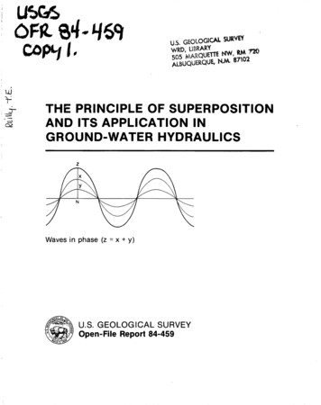
U.S. GEOLOG\CAL SURVEYWRD UBRARYno505 ,MARQUETTE tNI lMAlBUQUERQUE, N.M. 87102I1, .' tL.)r-&THE PRINCIPLE OF SUPERPOSITIONAND ITS APPLICATION INGROUND-WATER HYDRAULICSzWaves in phase (z x y)U.S. GEOLOGICAL SURVEYOpen-File Report 84-459
lJ.SGtSor- -.Lf6qC.Ju.s.GEOLOGICAl SURVEY.WRD L1 BRARY.SOS 'MARQUETTE NW, RM 720ALBUQUERQUE, N.M. 87102THE PRINCIPLE OF SUPERPOSITIONAND ITS APPLICATION INGROUN.D-WATER HYDRAULICSBy Thomas E. Reilly, 0. Lehn Franke, and Gordon D. BennettU.S. GEOLOGICAL SURVEYOpen-File Report 84-459
UNITED STATES DEPARTMENT OF THE INTERIORDONALD PAUL HODEL, SecretaryGEOLOGICAL SURVEYDallas L. Peck, DirectorFor additional informationwrite to:Copies of this report may bepurchased from:u.s. Geological SurveyBranch of Ground WaterMail Stop 411Reston, Virginia 22092Telephone: (703)860-6904Open-File Services SectionWestern Distribution Branchu.s. Geological SurveyBox 25425, Federal CenterDenver, Colorado 80225Telephone: (303)236-7476ii
CONTENTSPageAbstract IntroductionPurpose and scope Acknowledgments Linear systems and linear equations. Definition of superposition. Application of superposition to a simple hydrologic system Mathematical demonstration of superposition concept Boundary conditions, stresses, and initial conditions in modelsthat use superposition Problem 1. Exercise. Discussion. . Application of superposition in a well problem Advantages of superposition. Constraints on the use of superposition. Problem 2. Exercise. Discussion. Application of superposition to nonlinear systems.Summary and concluding remarks References cited Appendix 1: Discussion on the solution of differential equationsand the role of boundary conditions - 11222347812151616171818192325252627Appendix 2:Recognition of linear and nonlinear differential equations.30Appendix 3:Completed work sheets33ILLUSTRATIONSFigure 1.Diagrammatic representation of a system and its associatedstress and response 32.Diagram showing superposition of simple sound waves43.Diagram showing superposition of heads and flows in aone-dimensional example 5Diagram showing the plan view and cross section of a hypothetical aquifer and associated boundaries. 10Diagram showing aquifer system under study and headdistribution in response to stress: A, cross-sectional viewof aquifer system and boundaries; B, plan view of aquifer;C, head distribution before pumping; and D, drawdowns andchanges in flow due to pumping. 134.5.iii
ILLUSTRATIONS (continued)PageFigure 6.7.8.Diagram showing superposition of well solutions: A, initialpumpage starting at to and its resulting drawdown s1 at t2;B, change in pumpage from the initial rate starting at t1and its resulting drawdown s2 at t2; C, total pumpagestarting at initial rate and increasing at t1, and itsresulting drawdown s1 s2 at t2 as obtained bysuperposition 16Cross section of confined aquifer with one-dimensional flowinto stream, as described in problem 2. 19Example of solutions to a differential equation: A, diagramshowing idealized aquifer system; B, two of the family ofcurves solving the general differential equation for theidealized aquifer system. ·28WORK SHEETSPageWork sheet 1.2.3.4.Grid for calculation of new head distribution andflow rates. 15Calculation for question A of problem 2 (refer tofig. 7) 20A through E of problem 2. Table of heads and head changes calculated for questions 21Graph of heads and changes in heads at 2,000-ft intervalsfrom stream, as calculated in problem 2 24COMPLETED WORK SHEETS1 332 3 4353634. . . . . . . . . . . . . . . .iv
CONVERSION FACTORS AND ABBREVIATIONSMultiEl inch-Eound units!Y.To obtain metric (SI)1 unitscubic foot per second(ft3/s)0.0283cubic meter per second(m3/s)million gallons per day(Mgal/d)0.0438cubic meter per second(m3/s)mile (mi)1.609kilometer (km)foot (ft)0.3048meter (m)1 International System of units.v
vi
THE PRINCIPLE OF SUPERPOSITION AND ITS APPLICATIONINGROUND ATERHYDRAULICSby Thomas E. Reilly, 0. Lehn Franke, and Gordon D. BennettABSTRACTThe principle of superposition, a powerful mathematicaltechnique for analyzing certain types of complex problems in manyareas of science and technology, has important applications inground-water hydraulics and modeling of ground-water systems. Theprinciple of superposition states that problem solutions can beadded together to obtain composite solutions. This principleapplies to linear systems governed by linear differentialequations.This report introduces the principle of superposition as itapplies to ground-water hydrology and provides backgroundinformation, discussion, illustrative problems with solutions, andproblems to be solved by the reader.INTRODUCTIONThe principle of superposition in physics is a simple concept·that hasnumerous applications in ground-water hydraulics and modeling! of ground-watersystems. The theory of superposition, which states that the solutions toindividual parts of a problem can be added to solve composite problems, isexplained in most books on advanced calculus or differential equations.Several texts on ground water provide some discussion of this topic as well;Bear {1979) gives perhaps the most comprehensive treatment that is readily1 The word "model" is used in several different ways in this report and inground-water hydrology. A general definition of model is a representationof some or all of the properties of a system. Developing a "conceptualmodel" of the ground-:-water system is the first and critical step in anystudy, particularly studies involving mathematical-numerical modeling. Inthis context, a conceptual model is a clear, qualitative, physical pictureof how the natural system operates. A "mathematical model" represents thesystem under study through mathematical equations and procedures. Thedifferential equations that describe a physical process {for example,ground-water flow and solute transport) in approximate terms are amathematical model of that process. The solution to these differentialequations in a specific problem frequently requires numerical procedures{algorithms), although many simpler mathematical models can be solvedanalytically. Thus, the process of "modeling" usually implies eitherdeveloping a conceptual model, a mathematical model, or amathematical-numerical model of the system or problem under study. Thecontext will suggest which meaning of "model" is intended.1
available. Yet, many ground-water hydrologists who do not have a strongbackground in mathematics do not understand the concept of superposition norits application to ground-water problems, despite the fact that they often usethis principle, perhaps unknowingly, in the analysis of pumping tests1.Purpose and ScopeThe purpose of this report is to introduce the principle of superpositionto hydrologists by providing background ·information, discussion, and fourproblems to be solved by the reader. (Solutions are included.)The discussion and problems in this report are directed toward theanalysis and computer simulation of flow patterns within ground-water systemsthrough superposition. It is hoped that after serious study of this document,the reader will be prepared for practical application of this concept.The method of images, which is an important application of superpositionin ground-water hydraulics, is not discussed in this report but is discussedin some detail by Walton (1970, p. 157-167).AcknowledgmentsThe authors are deeply indebted to the other instructors of the course"Ground-Water Concepts," given at the U.S. Geological Survey's NationalTraining Center. Over the years, the training materials for this course,including this report, have been generated through a melding of the ideas andwork of many individuals including Eugene Patten, Ren Jen Sun, Edwin Weeks,and others.LINEAR SYSTEMS AND LINEAR EQUATIONSSuperposition applies to linear problems or linear systems. A simplediagrammatic representation of a system with its input (or stress acting uponit) and its output (or response) is shown in figure 1. Simply stated, in alinear system, dqubling a given stress (input) will double the response,halving the stress (input) will halve the response, and so on. For example, avertical spring fixed.firmly at its upper end represents a close approximationto a linear physical system. If we attach a 1-pound weight (the stress) tothe lower end of the spring (the system), the spring will elongate or displacesome distance equal to x. (This constitutes the system response.) . If weremove the 1-pound weight and substitute a 3-pound weight, the response willbe 3x, and so on.1 The first step in analyzing a pumping test is to convert absolute headmeasurements to drawdowns, which represent changes in head superposed on theground-water system in response to the pumping stress. This step isrequired because the analytical solutions to linear well hydraulic problemsare expressed in terms of head changes--that is, these solutions usesuperposition.2
InputorStress.OutputorResponseSYSTEM.Figure 1.- Diagrammatic representation of a systemand Its associated stress and response.Linear systems are described by linear mathematical equations. Theprevious example relating spring elongation to applied weight is describe-d bythe simple linear algebraic equationF -Kx,where:F is the force (weight) acting at the end of spring,x is the elongation of the spring (a length), andK'is a constant (the spring constant), which is a property of thespring.The flow of ground water is defined in the general case by partialdifferential equations. The solution to a ground-water problem entailssolving the governing partial differential equation and satisfying theboundary and initial conditions that define the particular problem. (Adetailed discussion on boundary and initial conditions is given in Franke,Reilly, and Bennett, 1984, and a discussion of the solution of differentialequations and the role of boundary conditions is given in appendix 1.) Someof the differential equations that describe ground-water flow are linear andsome nonlinear. Because superposition applies to linear systems that aredescribed by linear equations, the concept of the linearity (or nonlinearity)of a differential equation is important. This topic is briefly reviewed inappendix 2.DEFINITION OF SUPERPOSITIONThe principle of superposition means that for linear systems, thesolution to a problem involving multiple inputs (or stresses) is equal to thesum of the solutions to a set of simpler individual problems that form thecomposite problem. For example, suppose we want to know the shape of thesound wave generated by two sound waves interfering with each other. Thisshape can be determined by algebraically adding the two simple waves together,as in figure 2, where the darker wave is the resultant wave. Thus, the shapeof a composite sound wave can be calculated from only the shape of eachcomponent wave. This procedure is valid because the properties of the wavesin figure 2 are governed by linear differential equations.A more formal definition of superposition is that, if Y1 and Y2 are twosolutions to a linear differential equation with linear boundary conditions,then C1Y1 C2Y2 is also a solution, where C1 and C2 are constants.3
zB. Waves partly out of phaseA. Waves In phase (Z x y)EXPLANATIONSimple sound waveResultant waveC. Waves out of phaseFigure 2. -Superposition of simple soundwaves.(Modified from Jeans, 1968.)APPLICATION OF SUPERPOSITION TO A SIMPLE HYDROLOGIC SYSTEMJust as the amplitudes of two simple waves were added together in figure2 .to obtain the amplitude of the composite wave, two different potentiometricdistributions resulting from two separate stresses in a confined aquifer canbe added together to obtain the potentiometric distribution resulting from thesum of the two stresses. For example, the one-dimensional aquifer systemshown in figure 3 is bounded by a river on one side and a canal on the other.In example a, the river stage is at datum, and the canal stage is 200 ftabove datum; in example b, the river stage is 50 ft above datum, and the canalstage is at datum. If the head distribution in the aquifer is known fromfield measurements or numerical calculations for examples a and b, then thehead distribution in example c, where the river stage is at 50 ft and thecanal at 200 ft, can be obtained by adding the heads in examples a and b.If the heads in examples a and b can be superposed (added together) togive a solution for example c, then the sum of the gradients (the slope of theline describing the head) in examples a and b should also give the gradient inexample c. In example a, the gradient is 0.100, and in example b it is-0.025; the gradient in example c is the difference, 0.075. The gradient signconvention as used here is arbitrary; the point is that the gradients inexamples a and b are of opposite sign.Finally, if the gradients can be superposed, so can the flows. Thus, ifthe flow (Q) from the canal to the aquifer is 4 units in example a and is -1unit in example b, then the flow in example c will be their sum, 3 units.4
:I!::: (0200 100\JA/r-200w0Ill (· w.wr-rV'e"JA-Confining layer-0- 'SZB-100-0 wCANALRIVER0::: -;:::Confined aquifer.J (a- f - -Impermeable bedrock2000ftA(a)200150a from canal to river100 4 units501000canalriverDISTANCE, IN FEET,w.w200ciw150 I-5100r-(b) .0 ( a from canal to riverr- -1 unit50 f-.0 (w00I1000riverDISTANCE, IN FEET2000canal(c)200150a from canal to river100 aa ab 4-150 3 units00riverB1000DISTANCE, IN FEETFigure 3. -2000canalSuperposition of heads and flows in a one-dimensional example- A. Confined aquifer bounded by ariver and canal. B. Plots of head distribution under three conditions: (a) with river stage at datum (0 ft.) and canalstage at 200 ft. ; (b) with river stage at 50 ft. and canal stage at datum (0 ft.); (c) addition of heads in (a) and (b) toobtain head distribution with river stage at 50 ft. and canal stage at 200ft.5
This simple demonstration illustrates an important point insuperposition. When we think of superposition in relation to ground-waterproblems, we generally think of adding heads. The preceding discussionindicates, however, that not only heads, but also gradients and flows, areadditive.Application of Darcy's law, which describes the flow through the crosssection in figure 3, helps to explain mathematically the additive process asdescribed above. Darcy's law statesdh-KAdxQwhere:(1)Q quantity of water discharged through the cross section (ft3/s);K hydraulic conductivity (ft/s);Across-sectional area (ft2);x distance from the river (ft); andhhydraulic head (ft).Darcy's law is the governing differential equation for the system offigure 3. For example a, let Qa represent the flow through the aquifer andha(x) represent the solution to the differential equation (the hydraulichead), and, in example b, let Qb and hb represent the corresponding flow andhead.We define the sum of the head distributions for the two examples ashc(x); that ishc(x) ha(x) hb(x).(2)Applying Darcy's law to example a yields(3a)dha(x)Qa-I Adxand to example bdhb(x)Qb-KA(3b)dxAdding equations 3a and 3b givesdhaQa Qb -KAdhb(3c)-KAdxdxHowever, the sum of the two derivatives may be written as the derivative ofthe sum. Thus,d(ha hb) dhcdhadhb dxdxdx6dx.
Substituting this into equation 3c givesQa Qb -KA(4a)dxEquation 4a, like equations 3a and 3b, is a statement of Darcy's law. Ittells us that hc(x), the head distribution defined by ha(x) hb(x), mustsatisfy Darcy's law provided ha(x) and hb(x) satisfy it individually.Equation 4a also shows that the flow corresponding to the combined headdistribution is Qa Qb, the sum of the flows corresponding to the individualhead distribution. That is,where Qc is the flow for the combined case.used, flows as well as heads must be added.Thus, when superposition isMATHEMATICAL DEMONSTRATION OF SUPERPOSITION CONCEPTIn ground-water problems involving a linear governing equation (such astwo-dimensional confined flow), the effects of individual changes (orstresses) can be evaluated without the need to consider the other concurrentstresses on the system. To demonstrate this, consider a system governed bythe following partial differential equation, which describes nonequilibriumflow in two dimensions under confined conditions:: (rx ah ) :dXClydX(ry ah ) w s ahCly(5)dtIn equation 5, transmissivity in the x direction transmissivity in the y direction source or sink term (1/T);s storage coefficient (unitless);TxTyw(12/T);(12/T);and the coordinate directions, x and y, are alined with the principaldirections of aquifer transmissivity. Now suppose that a particular set ofinputs or stresses, which is designated wl, prevails in the aquifer (ingeneral, W1 is a function of position and time). A certain distribution ofhead in space and time, h1 (x,y,t), (or for brevity simply hl) is observed inresponse to these stresses. This head distribution must be such that when itis substituted into equation 5 together with the stress function wl, theequation is satisfied. That is, it must be true that(6a)must be valid.7
Now suppose the stresses are changed, so that corresponding to thefunction W1 in equation 6a there is a new function. W, which gives the changeor difference in the stress from W1 The new stress function is then W1 W,and corresponding to this new stress pattern there is a new head pattern, h1 h, where h represents the difference in head·, from h1, which is observed inresponse to the change in stress w. Like h1 and W1, h and W are, ing neral, functions of x,y, and t.Because the system is still governed by equation 5, the new headdistribution and the new stress function must also satisfy this equation; thatis, it must be true that-a (axTXa(h 1 ax h))a ( - Tyaya(h 1 h))ay w1 w s(6b)atAgain, by the principle that the derivative of a sum is equal to the sum ofthe individual derivatives, equation 6b can be written sat(7)Subtracting equation 6a from equation 7 givesa (a h) - a ( Ty -a h) Tx axaxayay ws(8)atThus h (x,y,t), the function describing the change in head caused by thestress change W, must itself satisfy the governing differential equation offlow when it is subs ituted into that equation together with w. It followsthat: (1) the governing differential equation can be solved only for the headchanges h corresponding to the stress changes W; (2) head changes, h(drawdowns), can be used to solve for aquifer parameters, such as Tx and Ty;and (3) in general, individual solutions to a linear partial differentialequation can be added to provide new solutions corresponding to a combinedstress.BOUNDARY CONDITIONS, STRESSES, AND INITIAL CONDITIONSIN MODELS THAT USE SUPERPOSITIONIn using superposition to solve ground-water flow problems, we aredealing in terms of changes in head (drawdown) and changes in flow rather thanabsolute values of head and flow. The natural hydrologic boundaries (namelyconstant head, constant flow, and leakage boundaries), and the initialconditions, must be represented in models (either conceptual, analytical,analog, or numerical) in terms of changes instead of the actual valuesobserved in the flow system. The key to proper definition of boundary andinitial conditions when using superposition in the simulation of ground-waterproblems is to keep in mind that the model is solving for changes in heads8
{drawdowns) and flows. Thus, to define the boundary conditions in a modelsimulation that uses superposition means representing the change in head orflow that will occur at these boundaries.In ground-water models that use superposition, boundary conditions areusually represented in the following manner {see Franke, Reilly, and Bennett,19&4, for further discussion of boundary conditions):Constant-head and specified-head boundaries are represented as zeropotential boundaries, corresponding to zero drawdown or head change. If theabsolute value of head does not change at these boundaries in the naturalsystem, the superposition model represents this boundary as having zerodrawdown or buildup of head. If, on the other hand, the purpose of thesimulation is to determine the effect on the ground-water system of a changein absolute head at one of these boundaries, then the absolute value of thischange in head, h {difference between two absolute heads) becomes the newvalue of constant head in the superposition model, and the other constant headand specified head boundaries that remain unchanged are represented as zerohead potential boundaries.Constant-flux boundaries are represented by zero change in flow--that is,as zero-flux boundaries in a superposition model because the assumption thatflow across these boundaries remains constant implies that change in flow iszero. For example, when we evaluate the response of an aquifer to a pumpingwell through superposition, we often assume that natural recharge does notchange and thus represent the boundary at which recharge occurs as a no-flowboundary. If, on the other hand, we wish to simulate the effect on theground-water system of a change in flux at one of these boundaries, then thevalue of this change in flux becomes the new value of constant flux at thisboundary in the superposition model, and we again represent the otherconstant-flux boundaries that remain unchanged as no-flow boundaries.Leakage across a confining unit from a constant head source {mixedboundary condition) is represented in superposition by maintaining the sourceat zero drawdown, or zero change in head. As a result, the flow through theconfining unit in the superposition model represents the change in flowthrough the unit in the natural system due to the stress.These concepts related to definition of boundary conditions insuperposition models will be further clarified in a series of examples. Aground-water system with its associated physical boundaries is depicted bothin plan view and cross section in figure 4. The values for areal recharge andlateral inflow to the aquifer from the northern bedrock hills represent bestestimates ·based on a water budget, a measured potentiometric surface in theaquifer, and an estimate of aquifer transmissivity. A model of this systembased on absolute heads would use the following six boundary conditions:{1) a constant head equal to 400 ft along the western lateral boundary{reservoir) of the aquifer; {2) a constant flux of 3 ft 3 /s distributed alongthe northern lateral aquifer boundary; {3) specified heads along the easternlateral aquifer boundary corresponding to the river stages in figure 4a; {4) astream surface or no-flow boundary along the southern impervious bedrockhills; {5) a stream surface or no-flow boundary on the bottom of the aquifer;and {6) a constant areally distributed flux of 2 ft/yr on the top surface ofthe aquifer. In the following examples, a hypothetical modeling problem for9
.Bedrock hills provide constant lateral flow3of ground water to aquifer equal to 3.0ft /s. ,:·:'···: . .:·.'.::: :::. ':: ::---;·. :,.: .;',:::·.:·,: .: : ::. :'. ::::.:.·, .:.;::.::·.:·: . ·.;: ::.:·. ::::::·, / :·. ::::.'·.::·: . :·::. :.:.:::·:··:· ;;;-Ia:0 a:wenwa:!;8."'"'0 II.Confined aquifer;;;NN0 /"'0;;;j i5 "'N a:NwI .·;: ]' -. . . :;::\ Na: 1\8MImpermeable bedrock hillsA. PLAN VIEWwEAreally distributed recharge equals 2.0ft/yrjjjljConfining layerRESERVOIRRIVERAquiferImpermeable b drockB. CROSS SECTIONFigure 4. -Plan view and cross section of a hypothetical aqu ifer and associated boundariesthe system depicted in figure 4 is presented and is followed by the definitionof the boundary conditions in a model that simulates the problem throughsuperposition.Example 1:We wish to investigate the effect of a pumping well on the system.In a superposition model, both the western ·lateral boundary(reservoir) and eastern lateral boundary (river) are representedas constant-head boundaries of zero potential. All otherboundaries are no flow.10
Example 2:We wish to investigate the effect on the system of raising thestage of the reservoir from 400 ft to 450 ft. In a superpositionmodel, the western boundary (reservoir) is represented as a constant potential of 50 ft, the eastern lateral boundary (river) asa constant potential of zero, and all other boundaries are noflow.Example 3:The lateral inflow to the aquifer from the northern bedrock hillsis uncertain. We wish to investigate the effect on the system ofincreasing this lateral inflow from 3 ft3/s to 4 ft3/s. In asuperposition model, this northern boundary is represented as aconstant-flux boundary with areally distributed inflow totaling 1ft3/s, the western boundary (reservoir) and eastern boundary(river) are constant head with zero potential, and all otherboundaries are no flow.Example 4:We wish to investigate the effect on the system of changing thestage (and slope) of the river surface along the eastern boundaryof the aquifer. The new values of stage at selected points are(a) 220 ft, (b) 240 ft, (c) 260 ft, (d) 280 ft, and (e) 300 ft.In a superposition model investigating these changes in stage, theeastern river boundary is a specified head boundary with potentials of 20 ft at a, 15 ft at b, 10 ft at c, 5 ft at d, and 0 ftat e. The western boundary (reservoir) has a constant potentialof zero, and all other boundaries are no flow.Each of these examples considers a single change in the definition ofsome aspect of the system boundaries or the stress acting on the system. Thetotal effect on the system of some combination of these individual changes (orother changes) may be obtained by adding algebraically the response of thesystem (changes in heads and flows in the various parts of the system) to theindividual changes. Note that we can investigate not only increases but alsodecreases in reservoir stage, river stage, lateral inflow, or areal rechargeas well as artificial recharge. We must, however, keep track of the referencevalues of the variables because it is the changes in these values that we aredefining and investigating.Stresses are represented in superposition models through the same logicas the representation of boundaries--that only changes in stress arerepresented. Suppose, for example, we wish to simulate only the effect of anadditional pumping well on a ground-water system that is already heavilystressed. The discharge of water from this pumping well represents the changein stress on the system that will be simulated, and drawdowns in response toonly this pumping are determined by the model through superposition.These same concepts apply also to a pumping-test analysis wherein thenatural system may have many stresses acting on it, but we are interested onlyin the effect of the test well. An early step in the test analysis is tocalculate drawdowns at all observation points as a function of time. Thesemeasured drawdowns may undergo a series of corrections to account for temporaltrends in ground-water levels in the area during the pumping test, barometriceffects, tidal effects, and so on. The purpose of these corrections is toobtain, finally, drawdown data that reflect only the effect of pumping at thetest well.11
In a model that uses superposition, the initial potential distribution isnormally taken as zero throughout the system, thus representing zero headchange or drawdown. The stresses represented in the model would then be anychanges in stress under consideration from the time represented by the initialcondition. When comparing drawdowns calculated by a model through superposition with field-measured drawdowns, we must remember that the calculateddrawdowns reflect only the changes in stress represented in the model. Thefield-measured drawdowns, however, may include changes in head resulting fromstresses that were affecting the system before the initial time represented inthe model. Thus, the drawdowns calculated by the model will be comparable tothe actual drawdowns only if the natural system was in equilibrium at theinitial time represented by the model. (See Franke, Reilly, and Bennett,1984, for further discussion of initial conditions.)The above discussion assumes that the reference head in all models thatuse superposition is a zero change in head (zero drawdown), and this is aimostalways true. However, because the principle of superposition states that anysolutions to linear differential equations can be added to obtain newsolutions, a reference head of zero drawdown is not a requirement--it issimply the most straightforward.PROBLEM 1A square confined aquifer with a uniform transmissivity of 1.SS x 10-2ft 2 /s is shown in figure S. The aquifer is bounded by two impermeable rockwalls and two surface-water bodies laterally and by two assumed impermeableboundaries above and below the aquifer. The surface-water bodies are a riverand a reservoir whose stages remain constant (fig. SA, SB). Thus, a constanthead is exerted by the surface-water bodies at their contact surfaces with theaquifer. The natural head distribution with the river stage at zero altitudeand the reservoir at 200 ft was calculated by a finite-difference model; theresulting head distribution is an approximate solution to the ground-waterflow equation (eq. S) and is shown in figure SC.A pumping rate of 3.1 ft3/s was then simulated for the
information, discussion, illustrative problems with solutions, and problems to be solved by the reader. INTRODUCTION The principle of superposition in physics is a simple concept·that has numerous applications in ground-water h