Transcription
June 9, 2010Computational HydraulicsJohn FentonTU Wien, Institut für Wasserbau und IngenieurhydrologieKarlsplatz 13/E222, A-1040 Wienfenton@kw.tuwien.ac.atAbstractThe aim is to give an understanding of the numerical approximation and solution of physical systems,especially in open channel hydraulics, but with more general application in hydraulics and fluidmechanics generally.The marriage of hydraulics and computations has not always been happy, and often unnecessarilycomplicated methods have been developed and used, when a little more computational sophisticationwould have shown the possibility of using rather simpler methods.This course considers a number of problems in hydraulics, and it is shown how general methods,based on computational theory and practice, can be used to give simple methods that can be used inpractice.Table of ContentsReferences.21.Introduction – numerical methods.42.Reservoir routing . . . . . . . . . . .2.1 The traditional "Modified Puls" method . .2.2 An alternative form of the governing equation2.3 Solution as a differential equation . . . .2.4 An example . . . . . . . . . . .456673.The equations of open channel hydraulics3.1 Mass conservation equation . .3.2 Momentum conservation equation3.3 The long wave equations . . . 8. 9. 9. 104.Steady uniform flow in prismatic channels. .4.1 Computation of normal depth. 11. 125.Steady gradually-varied flow – backwater computations. . . .5.1 The differential equation . . . . . . . . . . . .5.2 Properties of gradually-varied flow and the governing equations5.3 When we do not compute – approximate analytical solution .5.4 Numerical solution of the gradually-varied flow equation . . . . . . . . . . . . . .5.5 Traditional methods5.6 Comparison of schemes . . . . . . . . . . . .113131415161719
Computational Hydraulics6.7.8.John FentonModel equations and theory for computationalmechanics . . . . . . . . . . .6.1 The advection equation . . . . .6.2 Convergence, stability, and consistency. . . . .6.3 The diffusion equation6.4 Advection-diffusion combined . . .hydraulics and fluid.2121242628Wave and flood propagation in rivers and canals . . . . . . . . .7.1 Governing equations . . . . . . . . . . . . . . .7.2 Initial conditions . . . . . . . . . . . . . . . .7.3 Boundary conditions . . . . . . . . . . . . . . . . . . . . . . . . . .7.4 The method of characteristics7.5 The Preissmann Box scheme . . . . . . . . . . . . . . . . . . .7.6 Explicit Forward-Time-Centre-Space scheme7.7 The slow-change approximation – advection-diffusion and kinematictheories . . . . . . . . . . . . . . . . . . .30303334343637The analysis and use of stage and discharge measurements. . . .8.1 Stage discharge method . . . . . . . . . . . . .8.2 Stage-discharge-slope method . . . . . . . . . . .8.3 Looped rating curves – correcting for unsteady effects in obtainingdischarge from stage . . . . . . . . . . . . . . . . . . .8.4 The effects of bed roughness on rating curves. 41. 41. 45. 46. 49. 52Appendix AThe momentum equation simplified . 38ReferencesBarnes, H. H. (1967), Roughness characteristics of natural channels, Water-Supply Paper 1849, U.S. GeologicalSurvey.URL: http://il.water.usgs.gov/proj/nvalues/Chow, V. T. (1959), Open-channel Hydraulics, McGraw-Hill, New York.Chow, V. T., Maidment, D. R. & Mays, L. W. (1988), Applied Hydrology, McGraw-Hill, New York.Fenton, J. D. (1992), Reservoir routing, Hydrological Sciences Journal 37, 233–246.URL: outing.pdfFenton, J. D. (1999), Calculating hydrographs from stage records, in ‘Proc. 28th IAHR Congress, 22-27 August1999, Graz, Austria, published as compact disk’.URL: ting-hydrographs-from-stage-records.pdfFenton, J. D. (2001), Rating curves: Part 2 - Representation and approximation, in ‘Proc. Conf. on Hydraulicsin Civil Engng, Hobart, 28-30 Nov.’, Inst. Engnrs, Aust., pp. 319–328.URL: nton, J. D. (2010), Calculating resistance to flow in open channels, Technical report, Alternative HydraulicsPaper 2.URL: tance-to-flow-in-open-channels.pdfFenton, J. D. & Keller, R. J. (2001), The calculation of streamflow from measurements of stage, Technical Report01/6, Cooperative Research Centre for Catchment Hydrology, Melbourne.URL: 06.pdfHenderson, F. M. (1966), Open Channel Flow, Macmillan, New York.Herschy, R. W. (1995), Streamflow Measurement, second edn, Spon, London.Hicks, D. M. & Mason, P. D. (1991), Roughness Characteristics of New Zealand Rivers, DSIR Marine and Freshwater, Wellington.2
Computational HydraulicsJohn FentonLiggett, J. A. & Cunge, J. A. (1975), Numerical methods of solution of the unsteady flow equations, in K. Mahmood & V. Yevjevich, eds, ‘Unsteady Flow in Open Channels’, Vol. 1, Water Resources Publications,Fort Collins, chapter 4.Lighthill, M. J. & Whitham, G. B. (1955), On kinematic waves. I: Flood movement in long rivers, Proc. Roy.Soc. London A 229, 281–316.Roberson, J. A., Cassidy, J. J. & Chaudhry, M. H. (1988), Hydraulic Engineering, Houghton Mifflin, Boston.Samuels, P. G. (1989), Backwater lengths in rivers, Proc. Inst. Civ. Engrs, Part 2 87, 571–582.Simons, D. B. & Richardson, E. V. (1962), The effect of bed roughness on depth-discharge relations in alluvialchannels, Water-Supply Paper 1498-E, U.S. Geological Survey.Yakowitz, S. & Szidarovszky, F. (1989), An Introduction to Numerical Computations, Macmillan, New York.3
Computational Hydraulics1.John FentonIntroduction – numerical methodsIn the first part of the course we considered methods for common problems, including solutions of nonlinearequations; systems of equations; interpolation of data including piecewise polynomial interpolation; approximationof data; differentiation and integration; numerical solution of ordinary differential equations. The lecture notes areat URL: Numerical-Methods.pdf.For the remainder of the course we will be considering problems in hydraulics, largely open-channel hydraulics,and will be developing methods to solve those problems computationally. Initially the problems considered arethose where there is a single independent variable, and we solve ordinary differential equations, notably for calculating the passage of floods through reservoirs and for steady flow in open channels. Subsequently we considerunsteady river problems such that variation with space and time are involved, and we solve partial differentialequations. We consider model equations that describe important phenomena in hydraulics and fluid mechanics,and develop methods for them. Then these methods are carried over to the full equations of open channel hydraulics.It will be found that the methods developed here are based on general methods of computational mechanics,and are rather simpler than many methods used in computational hydraulics by large software companies andorganisations. It is hoped that these lectures will empower people and give them confidence that they can solveproblems for themselves, incorporating a spirit of modelling, and not be dependent on large software packageswhose properties are often spurious.2.Reservoir routingI(t)Surface Area A A ASurface Area Az η ηz ηQ(η(t), t)Figure 2-1. Reservoir or tank, showing surface level varying with inflow, determining the rate of outflowConsider the problem shown in figure 2-1, where a generally unsteady inflow rate I enters a reservoir or a storagetank, and we have to calculate what the outflow rate Q is, as a function of time t. The action of the reservoiris usually to store water, and to release it more slowly, so that the outflow is delayed and the maximum value isless than the maximum inflow. Some reservoirs, notably in urban areas, are installed just for this purpose, and arecalled detention reservoirs or storages.Also consider the volume conservation equation, stating that the rate of change of volume in a reservoir is equal tothe difference between inflow and outflow rates:dS I(t) Q(η(t), t),dt(2.1)in which S is the volume of water stored in the reservoir, t is time, I(t) is the volume rate of inflow, which is aknown function of time or known at points in time, and Q(η(t), t) is the volume rate of outflow, which is usually aknown function of the surface elevation η(t), itself a function of time as shown, and the extra dependence on timeis if the outflow device such as a weir or a gate is moved. The procedure of solving this differential equation iscalled Level-pool Routing.The process can be visualised as in figure 2-2. Initially it is assumed that the flow is steady, when outflow equalsthe inflow. Then, a flood comes down the river and the inflow increases substantially as shown. It is assumed thatthe spillway cannot cope with this increase and so the water level rises in the reservoir until at the point O whenthe outflow over the spillway now balances the inflow. At this point, where I Q, equation (2.1) gives dS/dt 0so that the surface elevation in the reservoir also has a maximum, and so does the outflow over the spillway, so thatthe outflow is a maximum when the inflow equals the outflow. After this, the inflow might reduce quickly, but it4
Computational HydraulicsJohn FentonInflow IDischargeOutflow QTime (t)Figure 2-2. Typical inflow and outflow hydrographs for a reservoirstill takes some time for the extra volume of water to leave the reservoir.2.1The traditional "Modified Puls" methodThe traditional method of solving the problem is to relate the storage volume S to the surface elevation η, whichcan be done from knowledge of the variation of the plan area A of the reservoir surface and evaluatingZ ηA(z) dz,(2.2)S(η) usually by a low-order numerical approximation for various surface elevations. Equation (2.1) can be then bewrittendS I(t) Q(S(η(t)), t),(2.3)dtso that it is an ordinary differential equation for S as a function of time t that could be solved numerically.It can be solved numerically by any one of a number of methods, of which the most elementary are very simple,such as Euler’s method. Strangely, the fact that the problem is merely one of solving a differential equation seemsnot to have been recognised. The traditional method of solving equation (2.3), described in almost all bookson hydrology, is unnecessarily complicated. The differential equation is approximated by a forward differenceapproximation of the derivative and then a trapezoidal approximation for the right side, so that it is writtenS(t ) S(t) 12(I(t) I(t )) 12(Q(S(t ), t ) Q(S(t), t)) ,where is a finite step in time. The equation can be re-arranged to give2S(t)2S(t ) Q(S(t ), t ) I(t) I(t ) Q(S(t), t) (2.4)At a particular time level t all the quantities on the right side can be evaluated. The equation is then a nonlinearequation for the single unknown quantity S(t ), the storage volume at the next time step, which appears transcendentally on the left side. There are several methods for solving such nonlinear equations and the solution is inprinciple not particularly difficult. However textbooks at an introductory level are forced to present procedures forsolving such equations (by graphical methods or by inverse interpolation) which tend to obscure with mathematical and numerical detail the underlying simplicity of reservoir routing. At an advanced level a number of practicaldifficulties may arise, such that in the solution of the nonlinear equation considerable attention may have to begiven to pathological cases. As the methods are iterative, several function evaluations of the right side of equation(2.4) are necessary at each time step.5
Computational Hydraulics2.2John FentonAn alternative form of the governing equationAnother form of the differential equation can be simply obtained. Figure 2-1 shows the reservoir or tank surface,showing the surface level initially at z η and the level some time later at z η η. Of course in the limit η 0 the change in storage dS is given bydS A(η),dη(2.5)in terms of the plan area A of the water surface at elevation η. Substituting into equation (2.1) an equivalent formof the storage equation is obtained:I(t) Q(η, t)dη f (t, η) ,dtA(η)(2.6)which is a differential equation for the surface elevation itself, and we have introduced the symbol f (.) for theright side of the equation. This equation has been presented by Chow, Maidment & Mays (1988, Section 8.3), andby Roberson, Cassidy & Chaudhry (1988, Section 10.7), but as a supplementary form to equation (2.3). In fact ithas advantages over that form, and this formulation is be preferred. It makes no use of the storage volume S, whichthen does not have to be calculated. Also, the dependence of outflow Q on surface elevation is usually a simpleexpression from a weir-flow formula or the like. Usually where outflow is via outlet pipes and spillways, it can beexpressed as a simple mathematical function of η, usually involving terms like (η zoutlet )1/2 and/or (η zcrest )3/2 ,where zoutlet is the elevation of the pipe or tailrace outlet to atmosphere and zcrest is the elevation of the spillwaycrest. The dependence on t can be obtained by specifying the vertical gate opening or valve characteristic as afunction of time, usually as a coefficient multiplying these powers of η. In general the η formulation requires atable for A and η, obtained from planimetric information from contour maps, to give A(η) by interpolation.2.3Solution as a differential equationThe lecturer (Fenton 1992) adopted the differential equation (2.6) and emphasised that it was just a differentialequation that could be solved by any method for differential equations, most much simpler than the modified Pulsmethod. When he presented it at a conference in Christchurch in New Zealand, a friend of his said at question time"But this is trivial! I always solve it like that. Doesn’t everybody?". The answer, then as now, was "strangely andregrettably, no".2.3.1Euler’s methodThis is the simplest but least-accurate of all methods, being of first-order accuracy only. It is¡ ¡ I(ti ) Q(η i , ti )ηi 1 ηi f (ti , η i ) O 2 η i O 2 ,A(ηi )(2.7)where we use the notation ηi η (i ) for the solution at time step i, and f (.) for the right side of the differentialequation as shown. This makes the presentation of the next higher approximation simpler.2.3.2Heun’s methodThe scheme is evaluated in two steps and can be written:η i 1η i 12.3.3 ηi f (ti , η i ) ,¡ ¡ ¡ ηi f (ti , η i ) f ti 1 , η i 1 O 2 .2(2.8a)(2.8b)Richardson extrapolationFor simple Euler time-stepping solutions of ordinary differential equations, if we perform two simulations, onewith a time step and then one with /2, we have that at any step a more accurate solution, denoted by η is¡ η (t) 2 η(t, /2) η(t, ) O 3 ,(2.9)where the numerical solution at time t has been shown as a function of the step. This is very simply implemented.6
Computational Hydraulics2.3.4John FentonHigher-order methodsAny method or software for solving ordinary differential equations can be used. Fenton (1992) considered several,including higher-order Runge-Kutta methods, but for most purposes those mentioned here are adequate.2.4An example22InflowOutflow — accurateEuler — large steps (200s)Euler — small steps (100s)Richardon 00Time (sec)400050006000Figure 2-3. Computational results for the routing of a sudden storm through a small detention reservoirConsider a small detention reservoir, square in plan, with dimensions 100m by 100m, with water level at the crestof a sharp-crested weir of length of b 4 m, where the outflow over the sharp-crested weir can be taken to be Q (η) 0.6 gbη 3/2 ,(2.10)where g 9.8 ms 2 .The surrounding land has a slope (V:H) of about 1:2, so that the length of a reservoir side is100 2 2 η, where η is the surface elevation relative to the weir crest, andA(η) (100 4η)2 .The inflow hydrograph is:I(t) Qmin (Qmax Qmin )µtTmaxe1 t/Tmax¶5,(2.11)where the event starts at t 0 with Qmin and has a maximum Qmax at t Tmax . This general form will be usefulthroughout this course, as it mimics a typical storm, with a sudden rise, and slower fall. In this example we considera typical sudden local storm event, with Qmin 1 m3 s 1 , and Qmax 20 m3 s 1 at Tmax 1800 s.The problem was solved with an accurate 4th-order Runge-Kutta scheme, and the results are shown as a solid lineon figure 2-3, to provide a basis for comparison. Next, Euler’s method (equation 2.7) was used with 30 steps of200 s, with results that are barely acceptable. Halving the time step to 100 s and taking 60 steps gave the betterresults shown. It seems, as expected from knowledge of the behaviour of the global error of the Euler method, thatit has been halved at each point. Next, applying Richardson extrapolation, equation (2.9), gave the results shownby the crosses. They almost coincide with the accurate solution, and cross the inflow hydrograph with an apparenthorizontal gradient, as required, whereas the less-accurate results do not. Overall, it seems that the simplest Eulermethod can be used, but is better together with Richardson extrapolation. In fact, there was nothing in this examplethat required large time steps – a simpler approach might have been just to take rather smaller steps.The role of the detention reservoir in reducing the maximum flow from 20 m3 s 1 to 14.7 m3 s 1 is clear. If onewanted a larger reduction, it would require a longer spillway. It is possible in practice that this problem might havebeen solved in an inverse sense, to determine the spillway length for a given maximum outflow.7
Computational Hydraulics3.John FentonThe equations of open channel hydraulicsIn a course preliminary to this one1 , we went to a lot of trouble to obtain the long-wave equations for rivers andcanals, making the general assumption that flow was essentially one-dimensional, observing that such channels aremuch longer than they are wide or deep, and that variation along the stream is gradual.i x xQAA AQ QzQbAbyQb QbAb AbxFigure 3-1. Elemental length of channel showing control volumesConsider Figure 3-1, showing an elemental slice of channel of length x with two stationary vertical faces acrossthe flow. It includes two different control volumes. The surface shown by solid lines includes the channel crosssection, but not the moveable bed, and is used for mass and momentum conservation of the channel flow. Thesurface shown by dotted lines contains the soil moving as bed load. Each is modelled separately, subject to a massconservation equation, and each to a relationship that determines the flux. In this course we will not consider themovement of soil.BAηzZPyFigure 3-2. Cross-section of channel showing important dimensionsThe most important dependent quantities that we need to calculate are Q, the discharge or volume flux, as shownin figure 3-1, and η, the elevation of the free surface, as shown in the cross-section in figure 3-2. The equationsthat will be considered are in terms of other geometric quantities shown on that figure: A – cross-sectional area B – top width of the surface P – the wetted perimeter around which the resistance to the flow acts. Z – the elevation of the bed at any point, which we will see appears only in determining the mean slope.In fact, it is surprising that so few geometric quantities are involved!1The lecture notes are available here: URL: iver-Engineering.pdf8
Computational Hydraulics3.1John FentonMass conservation equationIf rainfall, seepage, or tributaries contribute an inflow volume rate i per unit length of stream, the mass conservationequation can be obtained A Q i.(3.1) t xRemarkably for hydraulics, this is almost exact. The only approximation has been that the channel is straight. Thissay that if the discharge Q is varying along the stream, and/or if there is inflow i, then the cross-sectional area Awill change with time, to accommodate the volume required.We usually work in terms of water surface elevation stage η, which is easily measurable and which is practicallymore important. We make a significant assumption here, but one that is usually accurate: the water surface ishorizontal across the stream. Now, if the surface changes by an amount δη in an increment of time δt, then thearea changes by an amount δA B δη, where B is the width of the stream surface. Taking the usual limit of smallvariations in calculus, we obtain A/ t B η/ t, and the mass conservation equation can be writtenB η Q i. t x(3.2)This is a partial differential equation in terms of distance along the channel x and time t, for the surface elevationη(x, t), which we have assumed is horizontal across the channel, and the discharge Q(x, t).3.2Momentum conservation equationIf we consider the fluid momentum in the x direction in the elemental slice of the above figure, we obtain anotherpartial differential equation in x and t, which is surprisingly simple in view of the complexity of the problem:µ¶ QQ2 η Q Q .(3.3) β gA ΛP t xA xA2The terms are: Q/ t – comes from the rate of change of momentum in the control volume with time¡ βQ2 /A / x – comes from the variation of momentum flux due to fluid velocity along the channel. Thequantity β is an empirical coefficient, modelling the velocity distribution across the channel. It is about 1.05and in many places taken to be 1.0. gA η/ x – comes from the pressure forces in the water. The pressure distribution has been assumed to behydrostatic, such that pressure is proportional to the depth of water above any point. If the surface slopes,such that η/ x is finite (and almost always negative), then in the water, along any horizontal line, there is anet downstream pressure gradient, which when integrated over the channel section, gives this term. ΛP Q Q /A2 – we consider the resistance to motion in the channel as being caused by a shear force τ on theboundary, with Weisbach’s empirical formula:µ ¶2λQτ ρ,(3.4)8Awhere λ is the dimensionless Weisbach resistance factor, ρ is the density, and Q/A is the mean velocity alongthe pipe or channel. It is convenient for us to consider channels which are not very steep, to introduce theparameter Λ λ/8, and to integrate this stress around the wetted perimeter P , giving the result shown,where we have written Q Q rather than Q2 to allow for possible negative values of Q in tidal estuaries.In fact, equation (3.3) is not ready for use, as expanding the second term would give a contribution A/ x, andwe need to express this in terms of the free surface gradient. It can be shown thatµ¶ A η B S̃ ,(3.5) x x9
Computational HydraulicsJohn Fentonwhere the symbol S̃ for the mean downstream bed slope across the section has been introduced such thatZ Z1dy,S̃ B x(3.6)Bwhere the negative sign has been used such that in the usual case when Z decreases with x, this mean downstreambed slope at a section is positive. In the usual case where bed topography is poorly known, a reasonable localapproximation or assumption is made to give a value of S̃.3.3The long wave equationsThe momentum equation (3.3) can then be expressed in terms of η/ x. Writing it and the mass-conservationequation again, we have the pair of partial differential equations1 Qi η , tB xBµ¶Q Q Q QQ2 B ηQ2 B Q. 2β gA β 2 β 2 S̃ ΛP tA xA xAA2(3.7)(3.8)These are the long wave equations, sometimes called the Saint-Venant equations. They are the basis for most openchannel hydraulics.3.3.1Other resistance formulations – Chézy and Gauckler-Manning-StricklerThe simplest model of a river is that the channel is prismatic, the flow is steady ( / t 0) and it is uniform, witha constant bed and surface slope S0 such that η/ x S̃ S0 . The momentum equation (3.8) givesΛPQ2 gAS0 ,A2giving the Weisbach equation for steady uniform flowQ ArgAS0 .ΛP(3.9)Other (and more traditional) formulations of the resistance term include those of Chézy and Gauckler-ManningStrickler. For them to agree for steady uniform flow, Λ can be expressed in terms of the Chézy coefficient C, theManning coefficient n, and the Strickler coefficient kSt respectively, the latter two being in SI units:Λ gn2 P 1/3g P 1/3g 2 1/3 ,21/3CkSt AA(3.10)giving the familiar results for steady uniform flow (note that Chézy is the same form as Weisbach):rQA CS0Chézy :APµ ¶2/3 pµ ¶2/3 pQA1 AGauckler-Manning-Strickler :S0 kStS0 An PP3.3.2Conveyance and Friction SlopeIt is convenient to introduce the conveyance K, so that the resistance term in the momentum equations appears as ΛPQ Q Q Q gA 2 .A2KFrom equation (3.10), the various definitions of K becomerr1 A5/3g A3A3A5/3 k,K C StΛ PPn P 2/3P 2/3(3.11)(3.12)showing that is a convenient shorthand that includes the resistance coefficient of whatever law is being used, plus10
Computational HydraulicsJohn Fentoncross-sectional geometry terms. It has units of discharge, L3 T 1 .A simple and important result for steady uniform flow is thatpQ K0 S0 ,(3.13)where the subscript 0 denotes the conveyance corresponding to the normal depth h0 of the uniform flow.Many textbook presentations write the friction term in terms of a dimensionless quantity Sf Q Q /K 2 , calledthe "friction slope", possibly better known as "resistance slope", so that the resistance term in the momentumequations appears as gASf . It is also known as the "slope of the energy grade line", or the "head gradient", whichgives an uninformative and misleading picture, for in our momentum-based approach it is neither of those things.In textbook derivations of the steady equations Sf is actually calculated from the slope of the energy grade line,which it should not be.3.3.3The nature of the long wave equationsThey are a pair of equations that can be written as a vector evolution equation u u C r (u) , t xwhere u is the vector of unknowns, for example, [η, Q], C is a 2 2 matrix with algebraic coefficients, and r isthe vector of right side terms, due to inflow, slope, and resistance.It can be shown that the system is hyperbolic, although this mathematical terminology seems not very useful for us.The implication of that is that solutions are of a wave-like nature. We will see that the behaviour of disturbances ismore complicated than we might expect or is often stated. This arises because the right sides are functions of thedependent variables, that we have written here as r (u). In particular we will see that a common interpretation ofthe system in terms of characteristics, with the solution that of travelling waves with simple properties, is incorrect.The solution is actually more complicated: disturbances travel at speeds which depend on their length, and showdiffusion as well.4.Steady uniform flow in prismatic channelsSteady flow does not change with time; uniform flow is where the depth does not change along the waterway. Forthis to occur the channel properties also must not change along the stream, such that the channel is prismatic, andthis occurs only in constructed canals. However in rivers if we need to calculate a flow or depth, it is common to usea cross-section which is representative of the reach being considered, and to assume it constant for the approximateapplication of theory. This is the simplest problem we consider!The Weisbach and Chézy equations and the Gauckler-Manning-Strickler forms give formulae for the discharge Qin terms of resistance coefficient, slope S0 , area A, and wetted perimeter P :rrA3/2 p8g A3/2 pg A3/2 pS S0 C 1/2 S0(4.1)Weisbach-Chézy :Q 01/21/2λ PΛPPA5/3 p1 A5/3 pG-M-S :Q S kS0(4.2)0Stn P 2/3P 2/3in which both A and P are functions of the flow depth. Each equation show how flow increases with cross-sectionalarea and slope and decreases with wetted perimeter. The maximum depth is the normal depth, and determining itis a common problem.Trapezoidal sections:Most canals are excavated to a trapezoidal section, and this is often used as aconvenient approximation to river cross-sections too. In many of the problems in this course we will consider thecase of trapezoidal sections. We will introduce the terms defined in Figure 4-1: the bottom width is W , the depth ish, the top width is B, and the batter slope, defined to be the ratio of H:V dimensions is γ. From these the following11
Computational HydraulicsJohn FentonBh1PγWFigure 4-1. Trapezoidal section showing important dimensionsimportant section properties are easily obtained:B W 2γhA h (W γh)pP W 2 1 γ 2 h.Top width :Area :Wetted perimeter :(Ex. Obtain these relations).4.1Computation of normal depthIf the discharge, slope, and the appropriate roughness coefficient are known, any of equations (4.1)-(4.2) is atranscendental equation for the normal depth h, which can be solved by the methods for solving transcendentalequations described earlier.In the case of wide channels, (i.e. channels rather wider than they are deep, h ¿ B, which is a common case)neither the wetted perimeter P nor the breadth B vary much with depth h. Hence the quantity A(h)/h also doesnot vary strongly with h. Hence we can rewrite the G-M-S expression: 1 A5/3 (h) pS0 (A(h)/h)5/3Q h5/3 ,S 0n P 2/3 (h)nP 2/3 (h)where most of the variation with h is contained in the last term h5/3 , and by solving for that term we can re-writethe equation in a form suitable for direct iterationµ¶3/5
Computational Hydraulics John Fenton 1. Introduction – numerical methods In the first part of the course we considered methods for common problems