Transcription
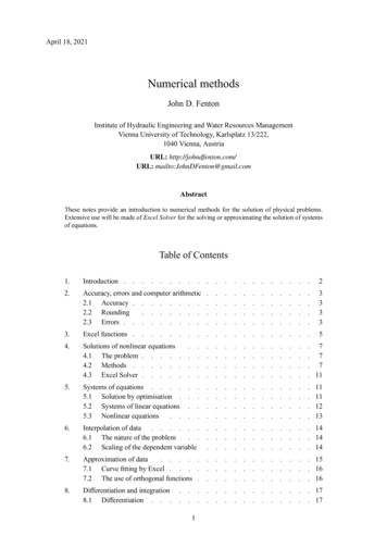
April 18, 2021Numerical methodsJohn D. FentonInstitute of Hydraulic Engineering and Water Resources ManagementVienna University of Technology, Karlsplatz 13/222,1040 Vienna, AustriaURL: http://johndfenton.com/URL: mailto:JohnDFenton@gmail.comAbstractThese notes provide an introduction to numerical methods for the solution of physical problems.Extensive use will be made of Excel Solver for the solving or approximating the solution of systemsof equations.Table of Contents1.Introduction .22.Accuracy, errors and computer arithmetic2.1 Accuracy . . . . . . . . . . . . . .2.2 Rounding2.3 Errors . . . . . . . . .33333.Excel functions .54.Solutions of nonlinear equations4.1 The problem . . . . .4.2 Methods . . . . . .4.3 Excel Solver . . . . . 7. 7. 7. 115.Systems of equations . . . .5.1 Solution by optimisation .5.2 Systems of linear equations5.3 Nonlinear equations . .6.Interpolation of data . . . . . . .6.1 The nature of the problem6.2 Scaling of the dependent variable. 14. 14. 147.Approximation of data. . . . .7.1 Curve fitting by Excel . . . .7.2 The use of orthogonal functions . 15. 16. 168.Differentiation and integration8.1 Differentiation . . . 17. 17.111111213
Numerical methods8.2John D. FentonIntegration. 189.Numerical solution of ordinary differential equations9.1 Euler’s method . . . . . . . . . .9.2 Higher-order schemes . . . . . . . .9.3 Higher-order differential equations . . . .9.4 Boundary value problems . . . . . . .10.Improved accuracy at almost no cost – Richardson & Aitken extrapolation .10.1 Richardson extrapolation . . . . . . . . . . . . . . . . . . . . . . . . . . . .10.2 Aitken’s 2 method. 25. 25. 2611.Piecewise polynomial interpolation – cubic splines . 2712.Piecewise polynomial approximation – cubic splines. 2913.A programming language – Visual Basic and Excel Macros13.1 Macros . . . . . . . . . . . . . .13.2 Visual Basic . . . . . . . . . . . . . 29. 29. 31. 33References.1919212223Accompanying documentsThe following Excel documents can be found in the same directory as this file:URL: and are referred to in the subsequent notes1.File nameDescription1-F UNCTIONS . XLSBasic Excel functions2-S OLUTION . XLSSolution of a single equation in a single variable3-S OLVER . XLSSolver applied to solution of equations, interpolation, and approximation4-F ITTING . XLSA curve fitting example where using Excel Trendline gave poor results5-D IFF - EQNS . XLSDifferent problems solved by different methods6-S PLINES . XLSUse of cubic splines for interpolationS PLINES . XLSContains the spline functions necessary for the previous spreadsheetIntroductionThrough the use of numerical methods many problems can be solved that would otherwise be thought to be insoluble. In the past, solving problems numerically often meant a great deal of programming and numerical problems.Programming languages such as Fortran, Basic, Pascal and C have been used extensively by scientists and engineers, but they are often difficult to program and to debug. Modern commonly-available software has gone a longway to overcoming such difficulties. Matlab, Maple, Mathematica, and MathCAD for example, are rather moreuser-friendly, as many operations have been modularised, such that the programmer can see rather more clearlywhat is going on. However, spreadsheet programs provide engineers and scientists with very powerful tools. Thetwo which will be referred to in these lectures are Microsoft Excel and Libre Office Calc. Spreadsheets are moreintuitive than using high-level languages, and one can easily learn to use a spreadsheet to a certain level. Yet oftenusers do not know how to translate powerful numerical procedures into spreadsheet calculations.It is the aim of these lectures to present the theory of the most useful numerical methods and to show how to implement them, usually in a spreadsheet, but occasionally also in a programming language, for sometimes spreadsheetsare not adequate for large-scale computations.The two spreadsheets we have mentioned are: Microsoft Excel – widely known and used. Some of its effectiveness for numerical computations comes from2
Numerical methodsJohn D. Fentona pair of modules, Goal Seek and Solver, which obviate the need for much programming and computations.Goal Seek, is easy to use, but it is limited – with it one can solve a single equation, however complicatedor however many spreadsheet cells are involved, whether the equation is linear or nonlinear. Solver is muchmore powerful. It was originally designed for optimisation problems, where one has to find values of anumber of different parameters such that some quantity is minimised, usually the sum of errors of a numberof equations. With this tool one can find such optimal solutions, or solutions of one or many equations, evenif they are nonlinear. In this course of lectures we will use it to simplify many procedures. It is somewhatannoying, however, that Solver is not automatically installed. You should open Excel, then click on the Toolstab. If Solver is not there you will have to click on Add-ins, and proceed to install it. Libre Office or OpenOffice Calc – Libre Office is a shareware version of Microsoft Office, with a wordprocessor, spreadsheet, presentation program, and drawing program; it can be downloaded from the site,https://www.libreoffice.org/. The package was originally Open Office, but that has not receivedmuch maintenance in recent years The spreadsheet is called Calc. It has most of the features of Excel,including Goal Seek, but at the time of writing, its version of Solver is not quite as good as that of Excel. Ituses a Genetic Algorithm, and is slower. In this course we will concentrate on Excel and will use that as ageneric name for the two programs.2.Accuracy, errors and computer arithmetic2.1AccuracyExcel stores and calculates with 15 digit accuracy. This is equivalent to double precision in some programminglanguages, and is accurate enough that most calculations do not suffer from significant loss of accuracy. Whenever10numbers are stored on a machine a small error usually occurs. Excel can store numbers in the range from 2 2 102 1024 10 308 to 22 21024 10308 . If the number is less than the minimum it stores it as 0, if greaterthan the maximum it records it as an overflow in the form #NUM!. Unlike programming languages, Excel does notdistinguish between integers and floating point numbers2.2Rounding Excel displays numbers rounded to the accuracy of the display. For example if you evaluate 2/3 and the cellhas been formatted to display 4 decimal places, it will appear as 0.6667. If you need to round a number there is a function ROUND(number,decimal places) which rounds anumber to a specified number of decimal places. If decimal places is 0, then the number is rounded tothe nearest integer, which is often useful in programming.Example: ROUND(3 14159 3) gives 3.142.2.3Errors1. Blunders: These are not really errors, but are mistakes, such as typing the wrong digit.2. Errors in the model: A mathematical model in civil and environmental engineering does not usually representevery aspect of a real problem, such as the neglect of turbulence in hydraulics.3. Errors in the data: Most data from a physical problem contain errors or uncertainties, due to the limitedaccuracy of the measuring device.4. Truncation error: This is the error made when a limiting process is truncated before one has reached thelimiting value such as when an infinite series is broken off after a finite number of terms.Example: computing sin from the first three terms of its power series expansion 3 3! 5 5!.5. Roundoff error: This is the error caused by the limited accuracy of the computer, and a roundoff error occurswhenever numbers are stored and arithmetic operations performed.In this course we will be concerned mainly with the last two types of errors.3
Numerical methods2.3.1John D. FentonAbsolute and relative errorsLet be the approximate value of a number whose exact value is .The absolute error in is .The relative error in is ( ) . The relative error is often given as a percentage.A number which is correct to decimal places has an error of less than 1 2 in the th decimal place,Absolute error 6 12 10 A number which is correct to significant digits has an error of less than 1 2 in the th digit,Relative error 6 12 101 Example: Consider 23 494 and 23 491. is correct to 4 significant figures and 2 decimal places: 0 003 12 0 00013 2.3.2 10 212 10 3 Roundoff error – an exampleIf we subtract two nearly equal numbers this leads to a loss of significant digits which can cause serious error ifused in further calculations. As an example, consider the quadratic formula for solving 2 0: 2 4 (2.1)2 and if is a large number, then 2 4 and subtracting the two to give the smaller root will be inaccuratedue to roundoff error. For example, take 1, 107 , and 1. Using Excel (with 15 figure accuracy) toevaluate the expression for the smaller root gives 0 9965 10 7 , which shows roundoff error. The correct answerto 15 figures is 1 10 7 .Some different proceduresHere as an example of different procedures we might adopt in other problemswe obtain the smaller root by different methods for the case 1, 107 , and 1. Note that we leave thebest method second!:1. As an example of the power and utility of Solver, and without requiring a great deal of mathematical orcomputational knowledge, Solver was used to obtain the root, by choosing an approximate small value of 0 and finding the solution of 2 107 1 0, which gave an answer of 1 00000000000001 10 7 ,correct to the full accuracy of Excel. The numerical optimisation method which Solver uses had no roundofferror problems here.2. In January 2019, John D. Sahr of Electrical and Computer Engineering at the University of Washington wrotea letter to the author, suggesting the following general and elegant solution. We should all use it as the standardalgorithm for solving a quadratic!It uses also the alternative solution of the quadratic that can be obtained by re-writing the quadratic 2 0 as 2 0, here solving for 1 using the usual formula, giving the alternative solutions 2 2 4 (2.2)Although this has the same problem, the solution liable to roundoff error here is for the other root, and so wecan use the algorithm 2 4 – If 0 compute 2 4 – If 0 compute – Then will no longer be the small difference of large numbers, and the two roots will be, first from theusual formula (2.1), then (2.2): 2 2 4
Numerical methodsJohn D. FentonExample 2.1 Using 6-figure arithmetic, solve the above example, 1, 107 , and 1: 0, 3.2 0 10 72 1 2 4 2 0 10 7 1 000000 10 7and22 0 10 7 1 000000 10 7 .Excel functionsAccompanying document Excel workbook 1-F UNCTIONS . XLS sets out the main commands which are necessaryat this stage. In the experience of the lecturer, Excel commands are accurate and robust although there has beensome discussion about some of the statistical routines.Figure 3-1. Elementary functions5
Numerical methodsJohn D. FentonFigure 3-2. Advanced functions6
Numerical methodsJohn D. Fenton4.Solutions of nonlinear equations4.1The problemThe problem is: if we have one equation in one unknown, and we need to find one, some, or all of the values ofthat unknown which satisfy the equation. That is, we have to solve ( ) 0, where ( ) is a known function of . This is finding the value of where the graph of ( ) intersects the axis. There may be more than onesolution.ExamplesA linear equation, with a simple solution 2. 2 0A quadratic – we might be able to factorise it, or use the formula for solving quadratics.2 4 3 0A higher degree polynomial – we might be able to factorise and solve, but in general it is unlikely 5 3 3 1 0A transcendental equation, which we are most unlikely to be able to solve.sin 1 0In the case of the last two equations we have to resort to numerical methods.4.2MethodsA number of different methods are presented here, for each has certain characteristics which favours its use incertain situations. For the purposes of this lecture course, however, we will see that Goal Seek and Solver are thesimplest and best to use, but in general any one of the others might have advantages.4.2.1Trial and errorThis involves simply guessing a value of , evaluate ( ), compare with zero, and then guess again. It is oftenused for one-off problems, but we often need to be much more systematic about it.4.2.2Newton’s method ( ) ( 0 ) ( ) 0 0 1 2 1 0 Figure 4-1. Newton’s methodThis method, if it converges, does so very quickly. Instead of just computing ( ), the derivative 0 ( ) is alsocalculated, and it is assumed that the next estimate of the root, or solution, is where the tangent crosses the axis.The values of ( ) and 0 ( ) there are calculated and the process repeated until it converges. The process is shownin figure 4-1, such that at iteration tan ( ) ( ) 0 ( ) 1from which an expression for the next estimate 1 is obtained 1 ( ) 0 ( )where ( ) 0 ( )(4.1)The convergence of this method is quadratic, such that the number of correct digits doubles at each step. However,7
Numerical methodsJohn D. Fentonif a double root occurs, such that the curve just touches the graph at the root and then curves away again, convergence is less rapid. Usually the correction at each stage ( ) 0 ( ) is calculated and monitored, andwhen it is less than a certain amount in magnitude, the process terminated.Example 4.1 With this method we can develop, for example, an algorithm to calculate the square root of anumber. Let the function ( ) 2 0, where is the number whose square root we want. Now, 0 ( ) 2 , and substituting into equation (4.1):¶µ 2 1 1 2 2 which is a simple and perhaps obvious algorithm: take the mean of your estimate and the number divided by thatquantity. Now, let’s find the square root of 100, starting with 100/2 as the first estimate:4.2.3Step 150 150 100 26 0250 110026 26 14 923 2 110014 923 14 923 10 8122 110010 812 10 812 10 03052 10010 0305 10 0305 10 0000512226 0314 923410 812510 030512The secant method ( ) ( ) 0 ( 0 ) ( 1 ) 3 2 1 0 Figure 4-2. Secant methodNewton’s method is unpleasant to apply if the function () is complicated, such that differentiation is a problem.In such cases it is appropriate to approximate the derivative by the secant approximation to the tangent. This meansthat 0 ( ) is approximated by 0 ( ) ( ) ( 1 ) ( ) ( 1 ) 1 1and the scheme requires two starting values ( 0 ( 0 )) and ( 1 ( 1 )) and it becomes 1 where ( ) 1 ( ) ( 1 )Example 4.2 We repeat the above problem using the secant method, using 0 and 50 as the first two estimates.Application of the method is shown in the following table.8
Numerical methodsJohn D. FentonStep 2 12 2 100 50150100 250050 48 02500 0100 22 48 1 84622 502100 3 8462 1 846 14 5753 8462 222350 48 0 2 02 1 846 3 846 99 9999790 000021 1010 0000000 000000Note that the method was somewhat slowly convergent as both numerator and denominator of the expression wentto zero in this special case. However, it still worked and the method has the decided advantage for complicatedfunctions that it is not necessary to obtain the derivative of the function.4.2.4Fixed point, direct, or simple iterationThis is a simple and obvious method and it is simple enough that if it works it can be very useful – but it goeswrong in about 50% of cases! We will investigate the conditions below. Once again, our problem is to solve theequation ( ) 0. However, if we can re-arrange this in the form ( ), where ( ) is some function of ,then this gives the scheme 1 ( ) meaning, assume some initial value 0 , evaluate ( 0 ) and use this value as the next estimate 1 and so on.Example 4.3 Use direct iteration to solve the equation 3 1 0.This obviously suggests the scheme 1 3 1. We start with 0 1: 3 1 13 1 0103 1 10 13 1 2 1 23 1 9 2 93 1 730 9It is obvious that the scheme is unstable and is not converging to a solution. Let us now try re-arranging theequation in the form: 1 ( 1)1 3 , with results: ( 1)1 3(1 1)1 3 1 25911 259(1 259 1)1 3 1 31211 3121(1 3121 1)1 3 1 32231 3223(1 3223 1)1 3 1 32431 3243(1 3243 1)1 3 1 3246It can be seen that the process is converging quite well.Why did one method work and not the other? The reason can be explained graphically, if we consider solving theequation ( ) to be equivalent to solving the pair of simultaneous equations and ( ) so that we plot the two graphs – the first is simply a straight line of gradient 1 passing through the origin, and theproblem is to determine where the second graph crosses it.The iteration procedure for different cases is shown in Figure 4-3. In Case A, the function has a gradient which isgreater than 1, and although we started near the solution at point 0, we were taken away from it. In the next Case Bthe function still has a negative slope, but it is less than 1 in magnitude and it can be seen how the solution spiralsin to converge. The last Case C is for a positive slope which is less than 1, and the process converges. These figures9
Numerical methodsJohn D. Fenton ( ) ( ) ( )000 0 Cases B and C: ( ) 1, stable0Case A: ( ) 1, unstableFigure 4-3. Unstable and stable behaviour of direct iteration scheme for different gradients of the functiondemonstrate the condition for convergence, that the direct iteration scheme 1 ( ) is stable if the gradientof the curve is less than one in magnitude in the vicinity of the root being sought, that is, ( ) 1 for stability. 4.2.5The bisection methodSuccessive intervals in which the solution lies012345 ( ) 0Figure 4-4. Bisection method, showing the successive halvings of the interval in which a solution is known to lieThis is a non-gradient method which uses a simple algorithm which can handle the most difficult of functions. Themethod will always converge to one solution provided a range which contains the solution is selected at the start.It proceeds by halving the range, then testing whether the solution is in the left or right half, and then repeating,halving the interval at each step. It is similar to a dictionary game, where one player selects a word, and anotherplayer has to guess the word by taking half the dictionary, asking if the word is in the first or second half of thedictionary, then in which half of that half and so on. If there are words, then it should be possible to get theword in tries, where 2 , or log2 . In the case of the a typical dictionary, with something like 80000words, log2 80000 16, i.e. 16 tries.The method is to bracket the solution initially, i.e. to find 0 and 0 such that the solution lies between the two,and then calculate the mid-point ( 0 0 ) 2 and by the sign of ( ), determine whether the solution isin the left or right half, and then to repeat until the interval is small enough. The algorithm can be written, where and are the left and right ends of the initial interval and is the required accuracy:10
Numerical methodsJohn D. Fenton ( ) ( )if( 0) exit and choose another or while ( ) ( ) 2 ( )if ( 0 ) else endifCalculate the values of the function at the endsThe function seems not to change sign in the intervalRepeat until the interval is small enoughCalculate the mid-pointCalculate the function thereDoes the sign of the function change in the left half?If so, reset the right boundary to the mid-pointOtherwise set the left boundary to the mid-pointThis method is not so easily programmed in a spreadsheet itself. Rather it is easily programmed in Visual Basic,the programming language which is available behind the spreadsheet. This can be accessed any time by usingAlt-F11 in Excel Workbook 2-S OLUTION . XLS.4.3Excel Solver84 ( ) 0-4-8-2-10 12Figure 4-5. Cubic function ( ) 3 1, with difficult behaviour for root-findingWorkbook 2-S OLUTION . XLS shows the use of Excel Solver to obtain the solution of a single equation in a singleunknown for the example used above, ( ) 3 1, to give an introduction to its use and to help us feelfamiliar with it. This simple cubic actually has a very nasty property, in that it has one solution, but the nature of thefunction, with a turning point where there is no solution is such as to throw off both Newton’s method and ExcelSolver, unless one starts sufficiently close to the solution. Plotting the function is always a good idea. Generally,however, using Excel Solver seems to be the best and simplest way of solving equations, most of which have ratherbetter properties than the example given.5.Systems of equations5.1Solution by optimisationSolver can be programmed to solve a much wider family of problems. It was originally designed for optimisationproblems, where one has to find values of a number of different parameters such that some quantity is minimised,usually the sum of errors of a number of equations. With this tool one can find such optimal solutions, or solutionsof one or many equations, even if they are nonlinear. All one has to do is to formulate the problem as one or moreequations.Let our system of equations be f (x) 0, where f and x are vectors such thatf (x) [ ( 1 ) 0 1 ] 11
Numerical methodsJohn D. Fentonnamely we have a system of equations in unknowns . If the equations are linear, a number of linearalgebra methods such as matrix inversion, etc. are possible, but the problems are usually more easily soluble withSolver. This even applies to the more general case, where the equations are nonlinear. In this process, , the sumof the squares of the errors for all the equations are evaluated: X 2 ( ) 1and the values of the found such that will be a minimum. If it should be possible to find a solutionsuch that 0 and the equations are solved. If there are fewer variables than equations, , then it will notbe possible to solve the equations, but minimising produces a useful solution anyway. This is particularly so inthe case of finding approximating functions.In the formulations of the present problems, we have to write all theequations with all terms taken over to one side, and then to implement an optimisation procedure such as Solver. Itdoes not matter how complicated the equations are – it is just necessary to be able to evaluate them. Most methodsfor minimising are gradient methods, such that in the -dimensional solution space, a direction is determined,and the minimum of the error function in that direction found, at the minimum a new direction found, usuallyorthogonal to the previous one, and so on. For two dimensions it can be shown as finding the minimum value ofa surface, as in Figure 5-1; the three dimensional case can be imagined as finding the hottest point in a room bysuccessively travelling in a number of different directions, finding the maximum in each, and then setting off atright angles, and so on. In either case the gradients are not obtained analytically but numerically by evaluating thefunctions at different values.Initial search pathMinimum on search (1)(1) 1 2Second search path Initialestimate(0)(0) 1 2Minimum desired ( 1 2 ) 2 1Figure 5-1. Typical search procedure to find a minimum – here a function of two variablesThis procedure usually means that we have simply to write down the equations, with initial trial values of theunknowns, and call the optimising routine. It is very general and powerful, and we can usually write down theequations in the simplest form, so that no algebraic manipulation is necessary or favourable. It can be seen that itworks simply, and no attention has to be paid to the solution process.5.2Systems of linear equationsVery commonly throughout engineering one encounters systems of linear simultaneous equations. These can besolved by direct methods such as Gaussian elimination, or LU decomposition into upper and lower triangular form.Computationally, a very popular method for 20 years has been Singular value decomposition, which also workswell on equations which are poorly conditioned, such that the solution is very sensitive to numerical accuracy. Ofcourse, other procedures for solving systems of linear equations are matrix methods, but these are often not ascomputationally efficient as the previously mentioned ones.Solver, however, can be used very simply to solve linear equations as well. An example is given in the Workbook3-S OLVER . XLS. This contains some simple examples in Worksheet L INEAR EQUATIONS. In the first example wecompare the use of typing out the equation with matrix notation.A well-conditioned system – two approachesConsider the system of equations 0 0 12 1 1 1
Numerical methodsJohn D. Fenton1. Firstly, the equations 1 0, 1 0, and 1 0 are typed and solved: 1, now eliminate from the first and third equations by adding to give 2 2, and back substitute 1 to give 0. Thissystem is well-conditioned, in that the solutions are not sensitive to numerical operations. Sometimes, whentwo or more of the three intersecting surfaces are very similar, the actual intersection point is poorly definedand the system is not well-conditioned.2. Whereas the writing and solution of the three equations was simple and obvious, it is sometimes easier towrite the equations as a matrix equation 1 0 1 1 0 1 0 1 1 0 1 1Solver can be used to actually solve the system of equations or to find the solution such that the sum of thea minimum. In this case Solver obtains the solution to six figures squares of the errors in each equation isT1.000000 1.000000 0.000000 .A singular system:in this case we consider 1 0 1 1 0 1 0 1 1 0 1 1where the last row is simply -1 times the first row. Solving this is equivalent to finding where one plane crossestwo planes which are coincident so that there is an infinityof solutions along a line where the planes T intersect, sothere is no unique solution. Solver found the solution 0 49999945 0 99999999 0 50000051 , and severalothers besides, just depending where the initial solution was.A poorly-conditioned system:in this case the system of equations is such that the system is not exactlysingular, but almost so, such that solutions depend very much on the numerical accuracy. Consider the examplewhich is simple but is notoriously poorly-conditioned: 1 12 31 41 1 1 1 1 1 1 12 31 41 51 1 34561111 14567In this case Solver had great trouble, and found a solution but with quite a large error, and it was not possible to refine this because of the poorly-conditioned nature of the system. It was interesting, however,that the matrix inverse T 460 180 140 .facility provided as part of Excel gave the correct solution correct to 16 decimal places,5.3Nonlinear equationsIn many physical problems, however, the system is not poorly conditioned, and Solver can obtain highly accuratesolutions. As it uses a scheme for minimising the sum of errors of a system of equations it does not matter whetherthe system is linear or nonlinear, which the next example in the spreadsheet shows.Example 5.1 Find where the parabola 2 crosses the circle 2 2 22 .In Solver we have two variable cells for and , plus a cell for the sum of the squares of the errors of the equations.However, it is usually clearer to set up a cell for the evaluation of each of the equations plus one cell where thesum of the squares is evaluated, and this is the cell that is minimised or solved. A single command can be used:SUMSQ(.). Here is the initial setup on Worksheet N ONLINEAR S YSTEMS in Workbook 3-S OLVER . XLS, with aninitial estimate of 1, 1:13
Numerical methodsJohn D. FentonColumn CColumn DSolutionRow 5 11Evaluate functions, each of which should be zero for a solutionMathematics:2 2 2 22Sum of squares:Excel contentsResultRow 9 C5-B5*B50Row 10 B5*B5 C5*C5-4-2Row 11 SUMSQ(D9:D10)4Now, running Solver with the Target Cell D11, Changeable Cells B5:C5, and seeking a Solution or Minimising thesum of the errors the method converges, 1 24962 , 1 56155 . Unpleasantly, with the initial solution 0, 0, it does not converge – so one has to be sufficiently close to a solution to converge to it. For problemsthat are not so nonlinear, this is not such a problem. Note this did not find another solution which was the negativeof both those numbers, unless an initial estimate of the solution closer to that one was assumed. If it finds onesolution, it provides no information as to how many exist or where the other ones are.Exercise:consider the problem of finding the intersection of the functio
Numericalmethods JohnD.Fenton slessrapid .