WIXLIB

A First Course in Hydraulics1.1.3John D. FentonDensityThe density is the mass per unit volume of the fluid. It may be considered as a point property of the fluid, and isthe limit of the ratio of the mass contained in a small volume to that volume: lim 0 In fact the limit introduced above must be used with caution. As we take the limit 0, the density behaves asshown in Figure 1-2. The real limit is , which for gases is the cube of the mean free path, and for liquidsis the volume of the molecule. For smaller volumes considered the fact that the fluid is actually an assemblage ofparticles becomes important. In this course we will assume that the fluid is continuous, the continuum hypothesis. If “inside” moleculePossible variation if the fluid is compressibleIf “outside” molecule V V *Figure 1-2. Density of a fluid as obtained by considering successively smaller volumes , showing the apparent limit of aconstant finite value at a point, but beyond which the continuum hypothesis breaks down.As the temperature of a fluid increases, the energy of the molecules as shown in Figure 1-1 increases, each moleculerequires more space, and the density decreases. This will be quantified below in §1.1.8, where it will be seen thatthe effect for water is small.1.1.4Surface tensionThis is an important determinant of the exchange processes between the air and water, such as, for example, thepurification of water in a reservoir, or the nature of violent flow down a spillway. For the purposes of this course itis not important and will not be considered further.1.1.5Bulk modulus and compressibility of fluidsThe effect of a pressure change is to bring about a compression or expansion of the fluid by an amount . Thetwo are related by the bulk modulus , constant for a constant temperature, defined: The latter term is the ”volumetric strain”. is large for liquids, so that density changes due to pressure changesmay be neglected in many cases. For water it is 2 070 G N m 2 . If the pressure of water is reduced from 1atmosphere (101,000 N m 2 ) to zero, the density is reduced by 0.005%. Thus, for many practical purposes wateris incompressible with change of pressure.1.1.6DiffusivityFluids may contain molecules of other materials, such as chemical pollutants. The existence of such materials ismeasured by the mass concentration per unit volume in a limiting sense as the measuring volume goes to zero. ata point, invoking the continuum hypothesis. The particles will behave rather similarly to individual fluid moleculesbut where they retain their identity, as suggested in Figure 1-1(c).Diffusion is the spontaneous spreading of matter (particles or molecules), heat, momentum, or light because of acontinuous process of random particle movements. No work is required for diffusion in a closed system. It is one6

A First Course in HydraulicsJohn D. Fentontype of transport process, which in many areas of water engineering is not important and can be neglected, yet it isresponsible for several important processes as well.Figure 1-3. Typical behaviour of diffusion of an initial point concentrationWe can consider a discrete physical analogy that reveals the nature of diffusion, but instead of a three-dimensionalmedium, a one-dimensional medium is considered, where a single particle is free to make a series of discretemovements, either to left or right, according to no particular physical law, merely the likelihood that the particlewill move and it can move in either direction. If we consider an initial cloud of many particles concentratednear a single point, it can be shown that this process proceeds as shown in Figure 1-3, where the concentration isplotted vertically as a function of horizontal distance . It shows the macroscopic behaviour of diffusion, whereirregularities and concentrations spread out as time passes, such that as time becomes infinite the diffusing quantityis everywhere but in vanishingly-small quantities. This is perhaps a surprising result, that in a cloud of particles,if a particle can go in any direction, the net result is for it to spread out. If we consider a region of uniformconcentration, say, then if any particle moves, it moves to the same concentration. On the edge of the cloud,however, a particle can move either back into the cloud, not changing the concentration, or it can move out of thecloud, thereby contributing to the spreading out of the cloud. At the next time step, this would be repeated, and soon.It can be shown that we obtain Fick’s law1 for the mass flux (flow) in the direction due to diffusion: (1.1)where is the coefficient of diffusion, of dimensions L2 T 1 , expressing the ease with which particles move throughthe surrounding medium. The negative sign is because particles flow from a region of high concentration to oneof low. Note that has units of concentration velocity, the rate at which matter is being transported per unitcross-sectional area of flow.Hence we have seen that the flow of matter is proportional to the gradient of the concentration – but that thisdoes not come from any special physical property of the concentration, such as particles being repelled by similarparticles, but merely because where there are many particles there will be more travelling away from that regionthan are travelling to that region. In all cases of diffusion, the net flux of the transported quantity (atoms, energy, orelectrons) is equal to a physical property (diffusivity, thermal conductivity, electrical conductivity) multiplied by agradient (a concentration, thermal, electric field gradient). Noticeable transport occurs only if there is a gradient- for example in thermal diffusion, if the temperature is constant, heat will move as quickly in one direction as inthe other, producing no net heat transport or change in temperature.In Brownian motion and diffusion the random motion comes from the molecular natures of the constituents. Belowit will be shown that in fluids this leads to the physical attribute of viscosity. Subsequently it is shown that in realpipes and waterways the random motion is dominated by the movement in the water of finite masses of water,rather than to individual molecules.1Adolf Fick (born 1829, in Kassel, Germany; died 1901), a medical doctor. He is usually credited withthe invention of contact lenses as well.7

A First Course in Hydraulics1.1.7John D. FentonViscosityIf, instead of the fluid being stationary in a mean sense, if parts of it are moving relative to other parts, then if afluid particle moves randomly, as shown above, it will in general move into a region of different velocity, therewill be some momentum transferred, and an apparent force or stress appears. This gives rise to the phenomenon ofviscosity, which is a diffusivity associated with the momentum or velocity of the moving fluid, and has the effectof smoothing out velocity gradients throughout the fluid in the same way that we saw that diffusivity of a substancein water leads to smoothing out of irregularities.A model of a viscous fluid:Consider two parallel moving rows of particles, each of mass , with ineach row. The bottom row is initially moving at velocity , the upper at , as shown in the figure. At a certaininstant, one particle moves, in the random fashion associated with the movement of molecules even in a still fluid,as shown earlier, from the lower to the upper row and another moves in the other direction.u uuThe velocities of the two rows after the exchange are written as and . Now considering the momenta of thetwo layers, the effect of the exchange of particles has been to increase the momentum of the slow row and decreasethat of the fast row. Hence there has been an apparent force across the interface, a shear stress.This can be quantified:Initial -momentum of bottom rowInitial -momentum of top rowChange of -momentum of bottom rowChange of -momentum of top rowFinal -momentum of bottom rowFinal -momentum of top row ( ) ( )( ) ( ) ( )( )In the absence of other forces, equating the momenta gives ( ) ( ) Thus, and Hence the lower slower fluid is moving slightly faster and the faster upper fluid is moving slightly slower thanbefore. Subtracting, the velocity difference between them now gives 2 thus and we can see the effect of viscosity in reducing differences throughout the fluid.In fact, if we consider the whole shear flow as shown in Figure 1-4, we can obtain an expression for shear stress inthe fluid in terms of the velocity gradient, as follows:Impulse of top row on bottom 8

A First Course in HydraulicsJohn D. FentondzzduxFigure 1-4. Shear flow, where the velocity in one direction is a function of the transverse velocity co-ordinate If is the average time between such momentum exchanges, thenmean shear force As the horizontal velocity is a function of , then if the two rows are apart, the differential of is and the mean shear stress per unit distance normal to the flow ismean shear stress mean shear force length 1 where is the mean particle spacing in . Now, , , and are characteristic of the fluid and not of theflow, and so we have mean shear stress the transverse velocity shear gradient. Fluids for which this holds are known as Newtonian Fluids, as are mostcommon fluids. The law is written (1.2) where is the coefficient of dynamic viscosity, which is defined here. Although we have only considered parallelflows here, the result has been found to apply throughout Newtonian fluid flow.Effects of viscosity:The law (equation 1.2) shows how a transverse shear flow gives rise to shear stresses,which acts, as suggested more immediately by the molecular argument above, so as to redistribute momentumthroughout a fluid. (Consider how stirring a bucket of water with a thin rod can bring all the water into rotation imagine trying to stir a fluid without viscosity!) If the fluid at the boundary of a flow has a certain specified velocity(i.e. momentum per unit mass), then viscosity acts so as to distribute that momentum throughout the fluid. This canbe shown by considering the entry of flow into a pipe as shown in Figure 1-5. On the pipe wall the fluid velocitymust be zero, as the molecules adhere to the wall. Immediately inside the pipe entrance the velocity differences arelarge, as viscosity has not yet had time to act, but as flow passes down the pipe viscosity acts so as to smooth outthe differences, until a balance is reached between the shear stresses set up by the viscosity, the driving pressuregradient, and the momentum of the fluid.Figure 1-5. Entry of viscous flow into a pipe, showing the effect of viscosity smoothing the initially discontinuous velocitydistribution9

A First Course in HydraulicsJohn D. FentonKinematic viscosity:In the above discussion we gave a physical explanation as to why . Inresisting applied forces (such as gravity or pressure) the response of the fluid is proportional to the density :Total net force mass acceleration so that ( terms involving velocity gradients) pressure terms (terms involving fluid accelerations) It can be seen that dividing by density shows that in the fundamental equation of motion the viscosity appears inthe ratio . This is the Kinematic viscosity : Typical values for air and water are such that air water 1 8 10 2 . However, air water 1 2 10 3 , andcalculating the ratio of the kinematic viscosities gives: air water 15 Hence we find that in its effect on the flow patterns, air is 15 times more viscous than water!However, the viscosities of both air and water are small (compared with honey) and are such that viscous effectsare usually confined to thin layers adjacent to boundaries. In the body of the flow viscosity in itself is unimportant,however it is the reason that flows which are large and/or fast enough become unstable and turbulent, so that insteadof single molecules transferring momentum, finite masses of water move irregularly through the flow redistributingmomentum, and tending to make flows more uniform. In most flows of water engineering significance, the effectsof turbulence are much greater than those of molecular viscosity.The relative unimportance of viscous terms in many hydraulic engineering flowsg sin g Figure 1-6. Hypothetical laminar flow in a river if molecular viscosity were importantWe consider a simple model to give us an idea of the importance of viscosity. In fact, we proceed naively, presuming no knowledge of actual river flows, but supposing – incorrectly as we will see – that the flow is laminar, suchthat it consists of layers of fluid of different velocity moving smoothly over each other in a macroscopic sense, allirregularities being at a molecular scale.Consider the hypothetical river as shown in Figure 1-6 with typical characteristics: 2 m deep, with a slope ofsin 10 4 , a surface velocity of 1 m s 1 , and a velocity on the bottom of 0, as fluid particles on a solid surfacedo not move. The stress on the bottom can be estimated using Newton’s law of viscosity, equation (1.2), assuminga constant velocity gradient as a rough approximation, to calculate the force due to molecular viscosity on thebottom of the stream, giving (1 0) 2 0 5 s 1 :Shear stress on bottom 1000 10 6 0 5 5 10 4 N m 2 Now we estimate the gravity force on a hypothetical volume in the water extending from the bed to the surface, and from this we obtain the mean stress component parallel to the bed. The vertical gravity force isvolume density depth plan area of the volume, so that the pressure due to gravity on the bottomis approximately (assuming 10) given by 1000 10 2 20000 N. The component parallel to the bed,10

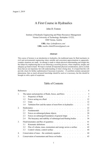
A First Course in HydraulicsJohn D. Fentonmultiplying by sin is 20000 10 4 2 0 N2 . Hence the ratio of viscosity/gravity 5 10 4 2 0 0 00025Hence, molecular viscosity is unimportant in determining the stresses.However, as we have considered all the forces acting parallel to the bed, and we have obtained a huge imbalancein the forces, our model seems defective. How can a typical river of these dimensions flow without the dominantgravity accelerating the flow hugely? The answer to this question will be presented in §1.4.2.1.1.8Typical values of physical properties of waterTemperature ( C) Density kg m 3Kinematic viscosity04102030 50 100999 81000999 7998 3995 7 988 958 11 7801 5841 3001 0060 805 0 556 0 294(units of 10 6 m2 s 1 )Table 1-2. Variation with temperature of the properties of pure water with no dissolved substances, from Jirka (2005) for the companion subject to thisThe density of water depends on temperature (see Table 1-2), dissolved solid concentration (especially salt), butlittle with pressure, as we have seen above. Changes in temperature and salinity are responsible for a number ofphenomena associated with convection currents and gravity currents, particularly in the ocean and lakes. Howeverin many fluid flows in rivers and pipes, these differences are small and can be ignored.Figure 1-7. Variation of gravitational acceleration ( m s 2 ) with latitude.Gravitational acceleration varies between 9 78 m s 2 at the equator and 9 83 m s 2 at the poles, so that studentscould use an appropriate value, as portrayed in Figure 1-7, however it is clear that a value of 9 8 m s 2 is accurateenough, and even a value of 10 m s 2 (correct to 2%) could be used with an accuracy commensurate with almostall of the theories and methods presented in this course.Density of fresh water 1000kg m 3Density of sea water 1025kg m 3Gravitational acceleration 9 8 10 6Kinematic viscosity 10m s 2m2 s 1Table 1-3. Typical values of physical properties associated with water problemsIn view of all the above remarks, in many engineering problems and in this course typical constant values can beassumed, which are set out in Table 1-3. It is a strange fact, and with the exception of the density of fresh water,an accidental one, that all of these quantities are close to an integer power of 10!2To have a feel for what a force specified in Newton is, 1 N is approximately the weight force on an apple!11

A First Course in Hydraulics1.2John D. FentonForces acting on a fluidn̂pdAgdA nˆ p m gDirectionForcemagnitude(a) Body force vector acting throughcentre of mass of fluid particle(b) Pressure force vector acting normalto local surface of fluidFigure 1-8. The two types of forces acting on a fluid particle – body force such as gravity acting through the centre of mass,and surface force, in this case pressure acting normally to the local surface.Consider figure 1-8 showing the two dominant types of forces acting on fluid particles.1. Body forces – this type of force acts at a distance, penetrating deep inside the fluid. - the most common isthat due to gravity. It is usually expressed as an acceleration, or, force per unit mass: Fbody g g where g is the acceleration due to gravity, g (0 0 ), where we have assumed that the co-ordinate isvertically upwards.2. Surface forcesa. Pressure forces – These are due to molecular motions of particles. Let n̂ be a unit vector normal to thesurface, directed into the fluid, then Fpressure n̂ Pressure is a scalar quantity. In a static fluid (one where all particles have the same velocity) there are noother stresses acting, and equilibrium of a finite volume leads to Pascal’s Law3 : pressure exerted anywherein a static fluid is transmitted equally in all directions.b. Shear forces – the relative motion of real fluids is accompanied by tangential stresses. Those due to viscous effects, whereby momentum exchange due to random movement of molecules occurs, are relativelysmall in hydraulics problems. Rather more important than that of individual molecules is the momentumexchange by turbulence and large masses of fluid.1.3UnitsThroughout we will use the Système Internationale, in terms of metres, kilograms and seconds, the fundamentalunits of mass (M), length (L) and time (T) respectively. Other quantities are derived from these. All are set out inTable 1-4. Some of the derived quantities will be described further below.1.41.4.1Turbulent flow and the nature of most flows in hydraulicsReynolds’ experiments (1883)Reynolds4 non-dimensionalised the differential equations which govern the flow of viscous fluid, and found that3Blaise Pascal (1623 – 1662) was a French mathematician, physicist, and religious philosopher, who made importantcontributions to the construction of mechanical calculators, the study of fluids, and clarified the concepts ofpressure and vacuum.4Osborne Reynolds (1842–1912) was a British engineering fluid dynamicist and professor of engineering at Manchester.12

A First Course in HydraulicsJohn D. FentonQuantitymasslengthtimetemperaturelinear velocityangular velocitylinear accelerationvolume flow ratemass flow ratelinear momentumforcework, energypowerpressure, stresssurface tensiondynamic viscositykinematic viscosityDimensionsUnitsFundamental quantitiesMkgLmTs C or K C 273 15Derived quantitiesLT 1m s 1 1Ts 1 2LTm s 2L3 T 1m3 s 1MT 1kg s 1 1MLTkg m s 1 2MLT1 kg m s 2 1 N (Newton)ML2 T 21 N m 1 J (Joule)1 J s 1 1 W (Watt)ML2 T 3 1 2ML T1 N m 2 1 Pa (Pascal) 10 5 bar 2MTN m 1ML 1 T 11 kg m 1 s 1 10 PoiseL2 T 11 m2 s 1 104 StokesTable 1-4. Quantities, d

A First Course in Hydraulics John D. Fenton References Batchelor, G. K. (1967), An Introduction to Fluid Dynamics, Cambridge. Colebrook, C. F. (1939), Turbulent flow in pipes with