Transcription
EE 410/510:Electromechanical SystemsT/Th 12:45 – 2:05 PM TH N155Instructor: J.D. Williams, Assistant ProfessorElectrical and Computer EngineeringU iUniversityit off AlAlabamabiin HHuntsvillet ill406 Optics Building, Huntsville, Al 35899Phone: (256) 824-2898, email: williams@eng.uah.eduCCoursematerialt i l postedt d on UAH AAngell course managementt websiteb itTextbook:S.E. Lyshevski, Electromechanical Systems and Devices, CRC Press, 2008ISBN Number: 978‐1‐4200‐6972‐3Optional Reading:H.D. Chai, Electromechanical Motion Devices, Prentice Hall, 1998S.J. Chapman, Electric Machinery Fundamentals, 4th ed. McGraw Hill, 2005S E Lyshevski,S.E.Lyshevski Engineering and Scientific Computations using MATLABMATLAB, WileyWiley, 2003A.E. Fitzgerald, C. Kingsley, S.D. Umans, Electric Machinery, 6th ed. McGraw Hill, 2003C.W. de Silva, Mechatronics: an Integrated Approach, CRC Press, 20045/21/20101All figures taken from primary textbook unless otherwise cited.
EE 410/510 - Electromechanical Systems:CCourseMMaterialt i l Chapter 1: Introduction to ElectromechanicalSystemsChapter 22. Analysis of ElectromechanicalSystems––– Modeling and Application of Op. Amps., PowerAmplifiers, and Power Converters––––Geometry and Equations of Motion GoverningDC Electric MotorsModeling and Simulation of DC Electric MotorsPermanent Magnet DC GeneratorDC Electric Machines with Power ElectronicsAxial Topology of DC Electric Machines andMagnetization CurrentsChapter 5. Induction Machines (someadvanced topics)––Overview 2 Phase AC Induction MotorsEquations of motion for 2 Phase AC Induction5/21/2010Motors– Torque Characteristics3 Phase induction motorsIntroduction to Quadrature and Direct VariablesArbitrary Reference FramesSimulation of 2 and 3 Phase AC Induction Motorsusing MATLAB and SimulinkChapter 6.6 Synchronous Machines (advancedtopic)–––Chapter 4. DC Electric Machines and MotorDevices– Review of ElectromagneticsReview of Classical MechanicsIntroduction to MATLAB and SimulinkChapter 3. Introduction to Power Electronics––––––IntroductionSingle and Three Phase Reluctance MotorsTwo and Three Phase Permanent MagnetgSynchronous Motors and Stepper MotorsMATLAB and Simulink SimulationsChapter 7. Introduction to Control ofElectromechanical Systems and PID ControlLaws–––Equations of Motion Governing the Dymamics ofElectromechanical SystemsAnalog PID Control laws and application involvingPermanent Magnet DC MotorDigital PID Control Laws and application involvingServosystem with Permanent Magnet DC Motor2
EE 410/510 - Electromechanical Systems:CCourseAAssignmentsitHomework:Homework will be assigned throughout the semester and is due 7 days afterassignment. Assignments will be graded and returned to account for 30% of thefinal course grade.gradeExams:Two in class exams will be given during the semester. Students will be allowedthe use of a calculator during the exam. All work will be performedindependently. Each exam will account for 25% of the student’s grade. The finalexam will be comprehensive covering major topics presented throughout thesemester and will constitute 20% of the course grade.Final Grade:HomeworkEExamsFinal5/21/2010Weekly2 per SSemestertComprehensive30%25%20%3
EE 410/510: Electromechanical SystemsChapters 1 and 2 ChapterCht 11: IIntroductiont d ti ttoElectromechanical SystemsChapter 2: Analysis of ElectromechanicalSystems and Devices Introduction to analysis and modeling Energy conversion and ForceProduction Overview of electromagnetics Overview of classical mechanics(Newtonian mechanics only) Applications of combined systems Simulation of systems in theMATLAB environment5/21/20104All figures taken from primary textbook unless otherwise cited.
Interdisciplinary Approach toEl tElectromechanicalh i i ti EKineticEnergyPotential Energy5/21/20105
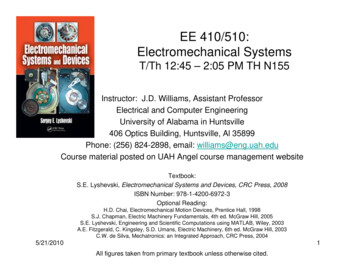
Modern Electromechanical Devices5/21/20106
Interdisciplinary Approach toEl tElectromechanicalh i lSSystemstEEngineeringii5/21/20107
Point Charge Distributions andC l b’ LCoulomb’sLaw The force, F, between two point charges Q1 and Q2 is:– Along the line joining them– Directly proportional to the product between them– Inversely proportional to the square of the distance between themQ1Q2F 4 o R 2Where k 14 o, o 8.854 10 12 C 2 / Nm 2– The equation above is easily calculated for a test charge, Q1, at theorigin and a source charge, Q2, at a distance R away.– The solution is slightly more complicated as we move our referenceframe away from the two charge such that Q1 is referenced by thevector r1 and Q2 is referenced by the r2r2.5/21/20108
Gauss’ LawGauss Gauss’ Law: The electric flux, , through any closed surface is equal to thetotal charge enclosed by that surface, thus QencIntegral Form D dS v dv QencsvApplying the divergence theorem, we have D dS D dv v dvsyielding the differential formvv D vThis is the first of the 4 Maxwell Equations which clearly states that thevolume charge density is equal to the divergence of the electric flux density5/21/2010Maxwell sMaxwell’sEquationsIn matter D v B E t B 0 D H J t9
Gauss’ Law(2)Gauss Gauss’ law is simply an alternative statement of Coulomb’s law.Gauss’ law provides an easy means of finding E or D for symmetrical chargedistributionsApplications: Point Charge D Dar 2dS ar r sin d d Qenc D dSs2 Qenc 2 Dar ar r sin d d 0 02 Qenc 22Drsin d d D4 r 0 05/21/2010 Q D a2 r4 rFigure from: M.N.O. Sadiku, Elements of Electromagnetics 4th ed. Oxford University Press, 2007.10
Electric Potential We define the electric potential (or the irrotational scalar field), V, describing anyelectrostaticl t t ti vectort field,fi ld E,E as theth magnitudeit d off ththe diffdifference betweenb tE att twotpoints a and b and some standard (common) reference point o. V ( p) E dlpnegativeega e by coconventione oob o V (b) V (a) E dl E dl E dlbo Now, the Gradient theorem states that dV E dl dV E cos dl dV Edl max5/21/2010 E VaaNote the crucial role that independenceof path plays: If E was dependent onpath, then the definition of V would benonsense because the path would alterthe value of V(p)11
The Dielectric Constant It is important to note that up to this point, we have not committed ourselves to thecause of the polarization, P. We dealt only with its effects. We have stated that thepolarization of a dielectric ordinary results from an electric field which lines up theatomic or molecular dipoles.In many substances, experimental evidence shows that the polarization is proportionalto the electric field, provided that E is not too strong. These substances are said tohave a linear, isotropic dielectric constantThis proportionality constant is called the electric susceptibility, e. The convention ist extracttot t theth permittivityitti it off ffree space fromftheth electricl t i susceptibilitytibilit tot makek theth unitsit dimensionless. Thus we have P o e E From the previous slide D o E P o (1 e ) E D o r E D E The dielectric constant (or relativepermittivity) of the material, r, is the ratioof the permittivity to that of free spaceIf the electric field is too strong, then it begins to strip electrons completely frommolecules leading conduction effects. This is called dielectric breakdown.The maximum strength of the electric that a dielectric can tolerate prior to whichbreakdown occurs is called the dielectric strength.5/21/201012
Using Gauss’Gauss Law With DielectricsTwo flat conductive plates ofarea Aarea,A, filled with dielectricConcentric Conducting Spheres withradius aa, b (b a) with a dielectric fillz - E1 s a z2 od Et E1 E2 s a z o E2 s a z2 o r- Dt Et o r Et r s a z D dS QencS D da DA QD QdV dl A a r Qa RE 4 o R 2 D V dl bb a Q4 o r r 2drQ 1 1 4 a b If capacitance, C Q/V, then what is the value for each example?5/21/201013Figure from: M.N.O. Sadiku, Elements of Electromagnetics 4th ed. Oxford University Press, 2007.
Continuity Equation Remembering that all charge is conserved, the time rate of decrease of chargewithin a given volume must be equal to the net outward flow through the surfaceof the volumeThus, the current out of a closed surface isApplying Stokes Theorem dQQ I J dS enclosed v dvd tdtSv v JdSJdv S v v t dv Continuity Equation J v tFor steady state problems, the derivative of charge with respect to time equalszero, and thus gradient of current density at the surface is zero, showing thatthere can be no net accumulation of charge.5/21/201014
Electrical Resistively Consider a conductor whose ends are maintained at a potential difference ( i.e. theelectricl t i fifieldld withinithi ththe conductord t iis nonzero andd a fifieldld iis passedd ththroughh ththe material.)t i l)Note that there is no static equilibrium in this system. The conductor is being fedenergy by the application of the electric field (bias potential)As electrons move within the material to set upp induction fields,, theyy scatter and aretherefore damped. This damping is quantified as the resistance, R, of the material.For this example assume:––a uniform cross sectional area S, and length l.The direction of the electric fieldfield, EE, produced is the same as the direction of flow of positivecharges (or the same as the current, I). E dl VR v I E dSsVlIVJ E Sl l 1VlR c I SS E 5/21/201015Figure from: M.N.O. Sadiku, Elements of Electromagnetics 4th ed. Oxford University Press, 2007.
Capacitance Capacitance is the ratio of the magnitude of charge on two separated platesto the potential difference between them Q E dSC V E dl Note that V E dl The negative sign is dropped in the definition abovebecause we are interested in the absolute value of the voltage dropCapacitance is obtained by one of two methods– Assuming Q, and determine V in terms of Q– Assuming V, and determine Q in terms of V If we use method 1, take the following steps – Choose a suitable coordinate system– Let the two conducting plates carry charges Q and –Q– Determine E using Coulomb’s or Gauss’s Law and find the magnitude ofthe voltage, V, via integration– Obtain C Q/V5/21/201016Figure from: M.N.O. Sadiku, Elements of Electromagnetics 4th ed. Oxford University Press, 2007.
Capacitance vs.vs Resistance E dlV R I E dS Q E dSR V E dlRC 5/21/2010C Sd,R d SParallel Plates b ln 2 LaCoaxial CylindersC ,R 2 L b ln a 1 1 4 a b Between 2 SpheresC ,R 4 1 1 a b 1Isolated SphereC 4 a, R 4 a17
Summary Diagram of Electrostatics V 14 o vrd E 2V v o14 o v arr2d E v o E 0 E VVE5/21/2010 V E dlFigure is recopied from Griffiths, Introduction to Electrodynamics,3rd ed., Benjamin Cummings, 1999.18
Biot-Savart’sot Sa a t s Lawa The differential magnetic field intensity, dH, produced at a point P, by the differentialcurrentt element,lt Idl,Idl isi proportionaltil tto ththe productd t Idl andd theth sinei off theth anglel bbetweentthe element and the line joining P to the element and is inversely proportional to thesquare of the distance, R, between P and the element Id l aˆ RId l RIdl sin dH 4 R 24 R 34 R 219Figure from: M.N.O. Sadiku, Elements of Electromagnetics 4th ed. Oxford University Press, 2007.
Ampere’spCircuit Law Ampere’s law: The line integral of H around a closed path is the same as the netcurrent, Ienc, enclosed by the path H d l I enc– Similar to Gauss’ law since Ampere’s law is easily used to determine H when thecurrent distribution is symmetrical– Ampere’s law ALWAYS holds, even if the current distribution is NOT symmetrical,however the equation is only used effectively for symmetric cases– Like Gauss and Coulomb’s Laws, Ampere’s aw is a special case of the Biot-Savartllawandd can bbe dderivedi d didirectlytl ffrom itit. Applying Stokes’s theorem provides alternative solution methodsI enc H dl J dSLI enc H dSSDefinition of Current provided in Chapter 5S H JMaxwell’s 3rd Eqn.20
DisplacementpCurrent Lets now examine time dependent fields from the perspective on Ampere’s Law. H J H 0 JThis vector identity for the cross product is mathematically valid. However, it requires that the continuity eqn. equals J v 0zero,, which is not valid from an electrostatics standpoint!p t Thus, lets add an additional current density term H J Jd to balance the electrostatic field requirement H 0 J Jd v D J d J D t t t DWe can now define the displacement current density asJd the time derivative of the displacement vector t D H J Another of Maxwell’s for time varying fields t This one relates Magnetic Field Intensity to conductionand displacementpcurrent densities5/21/201021
MagneticgFlux Densityy MagneticgFlux density,y B, is the magneticgequivalentqof the electric flux density, D. As such, one can defineB 0H 0 4 10 7 H / mwhere Similarly, Ampere’s Law is I enc B d lˆ0And the Magnetic flux through a surface is S B dS 0 H dSSThe magnetic flux through an enclosed system is S B dS B 0 B dvSDefinition of a solenoidal fieldand MaxwellMaxwell’ss 4th eqn.eqn22
Faraday’sFaradays Law (1) We have introduced several methods of examining magnetic fields in terms of forces,energy, and inductances.MMagneticti fieldsfi ld appear tto bbe a didirectt resultlt off chargehmovingi ththroughh a systemtandddemonstrate extremely similar field solutions for multipoles, and boundary conditionproblems.So is it not logical to attempt to model a magnetic field in terms of an electric one? This isthe question asked by Michael Faraday and Joseph Henry in 18311831. The result is Faraday’sFaraday sLaw for induced emfInduced electromotive force (emf) (in volts) in any closed circuit is equal to the time rate ofchangeg of magneticgflux byy the circuitVemf d d Ndtdtwhere, as before, is the flux linkage, is the magnetic flux, N is the number of turns in theinductor,, and t representspa time interval. The negativegsigng shows that the induced voltagegacts to oppose the flux producing it.The statement in blue above is known as Lenz’s Law: the induced voltage acts to oppose theflux producing it.Examples of emf generated electric fields: electric generators, batteries, thermocouples, fuelcells, photovoltaic cells, transformers.5/21/201023
Faraday’sFaradays Law (2) To elaborate on emf, lets consider a battery circuit. The electrochemical action within results and in emf produced electric field, Ef Acuminated charges at the terminals provide an electrostatic field Ee that also existthat counteracts the emf generated potential E E f EeP E dl E f dl 0 E f dl IRL LNThe total emf generated in by a time dependent motion or magnetic field is dBVemff E dl u B dldt LLS dB Em u Bdt Note the followingg importantpfacts An electrostatic field cannot maintain a steady current in a close circuit since E e dl 0 IRL An emfemf-producedproduced field is nonconservativeExcept in electrostatics, voltage and potential differences are usually not equivalent5/21/201024Figure from: M.N.O. Sadiku, Elements of Electromagnetics 4th ed. Oxford University Press, 2007.
Inductors and Inductance We now know that closed magnetic circuit carrying current I produces amagnetic field with flux B dS We define the flux linkage between a circuit with N identical turns as N As long as the medium the flux passes through is linear (isotropic) then thenflux linkage is proportional to the current I producing it and can be written as LI Where L is a constant of proportionality called the inductance of the circuit.A circuit that contains inductance is said to be an inductor.O can equateOnet theth iinductanced ttto ththe magneticti flflux off ththe circuiti it asL I N Iwhere L is measured in units of Henrys (H) Wb/AThe magnetic energy (in Joules) stored by the inductor is expressed as5/21/2010Wm 1LI22Figure from: M.N.O. Sadiku, Elements of Electromagnetics 4th ed. Oxford University Press, 2007.25
Inductors and Inductance Since we know that magnetic fields produce forces on nearby current elements, and that thosemagnetic fields can be generated by an isolated or coupled set of current carrying circuits, thenit is onlyy reasonable that such circuits mayy induce fields and magnetizationgbetween them We can calculate the individual flux linkage between the two components as 12 B2 dSS1 LikewiseLiki we can ddetermineti a mutualt l iinductanced tbbetweentththe circuitsi it ththatt iis equall ffrom circuiti it 12 12N 1 12as it is from circuit 21 asM 12 I2I2 Individual inductances are N N L1 11 1 1L 2 22 2 2I1I1I2I2 The total magnetic energy in the circuit is111W m W1 W 2 W12 L1 I 12 L 2 I 22 M 12 I 1 I 25/21/2010222Figure from: M.N.O. Sadiku, Elements of Electromagnetics 4th ed. Oxford University Press, 2007.26
Inductors and Inductance (2) As we eluded to before, you should think of an inductor as a conductor shaped in such a way asto store magnetic energyTypical examples include toroidstoroids, solenoidssolenoids, coaxial transmission lineslines, and parallel-wireparallel wiretransmission linesOne can determine the inductance for a given geometry using the following technique– Choose a suitable coordinate system– Let the inductor carry currentcurrent, I– Determine B from Biot-Savart’s or Amperes Law and calculate the magnetic flux– Find L as a function of the flux times the number of turns over the current carriedMutual inductance may be calculated by a similar approach– Determine the internal inductanceinductance, Lin for the flux generated by the first inductor– Determine the external inductance, Lext produced by the flux external of the first inductor– The sum of the internal and external inductance equals the individual inductances plus themutual inductance between the elements M 12 12I2 N 1 12I2 12 B2 dSS1For circuit theory, we can also right the inductance as which provides a very useful equationwhen quickly mapping out electronic circuits L extt C 5/21/2010 R L ext RC 1R L ext 27
Forces Due to a Magnetic Field Recall that the force on a charged particle is simply F qEIf the particle moves howeverhowever, then an additional force is imposed from the chargedisplacement of velocity, u, quantified by the magnetic field, B. The combinedforce is called the Lorentz Law: F q( E u B) Recall from Newton’s Law that The kinetic energy of a charged particlein an magnetic field is therefore duF q ( E u B) ma mddt5/21/2010 duF q (v B ) mdt q ( v y Bz v y Bz )q (v B ) xdtux dt mm q (v B ) yq ( v x Bz v z Bx )dt dtuy mm q ( v x B y v y Bx )q (v B ) zuz dt dtmm1 2KE m u2For B, u, and a in orthogonal directions,One can deduce a coordinatesystem in which qv B q(v B)1u1 dt dt v dtmm qBq (v B ) 2dt u1 uˆ2u2 mm q (v B ) 3Cyclotron Resonancedt 0u3 FrequencymThe location of the particle can also be found as dl28li ui dtu dt
Lorentz Force Law Recall that the force on a charged particle is simply F qEIf the particle moves howeverhowever, then an additional force is imposed from the chargedisplacement of velocity, u, quantified by the magnetic field, B. The combinedforce is called the Lorentz Law: F q( E u B) Recall from Newton’s Law that The kinetic energy of a charged particlein an electric field is therefore duF q ( E u B) ma mddt5/21/2010 duF q(E ) mdtqE xux dtmqE yuy dtmqE zuz dtm 21KE m u2The location of the particle can alsobe found as dlu dtli ui dt29
Magnetic Torque and Moment Now that we have examined the force on a current carrying loop. Let’s examine the Torqueapplied to itTorque, T, on the loop is the vector product of the force, F, and the moment arm, r. and for uniform B F0 IBl T IBlw sin butlw Syielding T IBS sin T r F T r F sin where 0 lF Idl B I dzaˆ z B dzaˆ z B F0 F0 0Ll 0 5/21/2010Where we can now define a quantity m asthe magnetic dipole moment with units A/m2which is the product of the current and areaof the loop in the direction normal the surfacearea defined by the loop m IS aˆ n T m BFigure from: M.N.O. Sadiku, Elements of Electromagnetics 4th ed. Oxford University Press, 2007.30
Torque and Dipole Propertiesoff a BarB MagnetMt A bar magnet or small filament loop is generally referred to as a magnetic dipoleAAssumeabbar magneticti off llength,th ll, generatest a uniformifmagneticti fifield,ld B,B andd a didipolelmoment, m QmlTorque, T, on the loop is the vector product of the force, F, and the moment arm, r.Thus, because the bar magnet represents aThusmagnetic dipole moment equal in magnitudeto the dipole moment of a current loop, a barmagnet can also be taken as a magneticdipole T m B Qml B F Qm B T QmlB ISB Qml IS5/21/2010Therefore the field at a reasonable distanceaway from any bar magnet is mathematicallyidentical to that of a dipole.Figure from: M.N.O. Sadiku, Elements of Electromagnetics 4th ed. Oxford University Press, 2007.31
Maxwell’sMaxwells EqnsEqns. for Static FieldsDifferential Form D vIntegral FormRemarks D dS v dvGauss’s Law B dS 0Nonexistence of theMagnetic Monopole E dl 0Conservative natureof the Electric Field H dl J dSAmpere’sAmperes LawS B 0S E 0L H JL5/21/2010S32
Maxwell’s Time Dependent Equations It was James Clark Maxwell that put all of this together and reduced electromagnetic fieldtheory to 4 simple equations. It was only through this clarification that the discovery ofelectromagnetic waves were discovered and the theory of light was developed.The equations Maxwell is credited with to completely describe any electromagnetic field(either statically or dynamically) are written as:Differential Form D vIntegral FormRemarks D dS v dvGauss’s LawS B 0 B E t D H J t5/21/2010 B dS 0Nonexistence of theMagnetic MonopoleS L E dl t S B dS D L H dl S J t dSFaraday’sFaradays LawAmpere’s Circuit Law33
Analogya ogy Betweenet ee Electricect c aandd Magneticag et c Fieldse dsElectric Basic Laws Force LawSource ElementField intensityFlux densityRelationship Between Fields Potentials Q 1Q 1aˆ rF 4 r 2 D dS Q enc F QEdQV(V / m )E l D C /m2S D E E V V FluxEnergy DensityPoisson’s Eqn. L dl4 r D dS Q CVdVI Cdt1 wE D E2 V v 2Magnetic Idl aˆ rdB 04 R 2 H dl I enc F Qu B Q u Id lI(A /m)H l B Wb / m 2S B H H V m , ( J 0 ) Id lA 4 R B dS LIdIdt1 wE B H2 2 A JI L34
Electromagnetic Work and Power 2 We 1 2 1D E E D we limElectric energy density v 0 v222 Wm 11 B 2 Magnetic energy density2 H H B wm lim v 0 v222 wT we wm1 W wT dv D E H B dv Electromagnetic energy2 2 1 P E H dS D E H B dv E dv t 2Sv Total electromagnetic power rate of decrease in stored energy – ohmic power dissipated5/21/201035
Electrostatic Boundary Conditions Electrostatic boundary conditions for E and D crossing any material interface mustmatch the following conditions developed using Guass’sGuass s law and conservation of theelectric fieldTwo different dielectrics characterized by 1 and 2. D v D dS QencSD1n D2 nE1n 1 E2 n 25/21/2010 E 0 E dlD1t 1 D2t 2E1t E2tFigure from: M.N.O. Sadiku, Elements of Electromagnetics 4th ed. Oxford University Press, 2007.36
Magnetic Boundary Conditions Magnetic boundary conditions for B and H crossing any material interface must match thefollowing conditions developed using Guass’sGuass s law for magnetic fields and Ampere’sAmpere s circuit law B dS 0 H dl I H dl I B1 n B 2 n 1 H 1n 2 H 2 n5/21/2010 H 1t H 2 t B1tB 2t 1 2Figure from: M.N.O. Sadiku, Elements of Electromagnetics 4th ed. Oxford University Press, 2007.37
Maxwell’s Time Dependent Equations:Identity Map5/21/201038Figure from: M.N.O. Sadiku, Elements of Electromagnetics 4th ed. Oxford University Press, 2007.
Classification of Magnetic Materials (1) In general we use the magnetic susceptibility (or relative permeability) to classify materials interms of their magnetic propertyA material is said to be nonmagnetic if there is no bound current density or zerosusceptibility. Otherwise it is magneticMagnetic materials may be grouped into three classes, diamagnetic, paramagnetic, andferromagneticFor many practice purposes, diamagnetic and paramagnetic materials exhibit little to nomagnetic susceptibility. What magnetic properties these materials do have follows a linearresponse over a large range of applied fieldsgmaterials keptp below the Curie temperaturepexhibit veryy largeg nonlinearFerromagneticmagnetic susceptibility and are used for conventional magnetic device applications5/21/201039Figure from: M.N.O. Sadiku, Elements of Electromagnetics 4th ed. Oxford University Press, 2007.
Classification of Magnetic Materials (2) Diamagnetism– Occurs when the magnetic fields in the material due to individual electron momentscancels each other outout. Thus the permanent magnetic moment of each atom is zerozero.– Such materials are very weakly affected by magnetic fields.– Diamagnetic materials include Copper, Bismuth, silicon, diamond, and sodium chloride(table salt)– In general this effect is temperature independentindependent. Thus,Thus for exampleexample, there is notechnique for magnetizing copper– Superconductors exhibit perfect diamagnetism. The effect is so strong that magneticfields applied across a superconductor do not penetrate more than a few atomic layers,resulting in B 0 within the materialParamagnetism– Materials whose atoms exhibit a slight non-zero magnetic moment– Paramangetism is temperature dependent– Most materials ((air,, tungsten,g, potassium,p, monell)) exhibit paramagneticpgeffects that pprovideslight magnetization in the presence of large fields at low temperatures5/21/201040
Classification of Magnetic Materials (3) Ferromagnetism–––––––Occurs inOi atomstwithith a relativelyl ti l llarge magneticti momenttExamples: Cobalt, Iron, Nickel, various alloys based on these threeCapable of being magnetized very strongly by a magnetic fieldRetain a considerable amount of their magnetization when removed from the fieldLose their ferromagneticgppropertiespand become linear pparamagneticgmaterials ((non magnetic)g) when thetemperature is raised above a critical temperature called the Curie temperature.Their magnetization is nonlinear. Thus the constitutive relation B 0 rH does not hold because rdepends directly on B and cannot be represented by a single value.Ferromagnetic shielding Ferromagnetic materials can be used to “focus” and guide the flow of incident magnetic fields By placing a ferromagnetic material completely around a device, one can shield said device froman external field. This shielding occurs b/c the ferromagnet acts as a magnetic waveguide, thattransmits the field around the shape of the structure and not within itit.5/21/201041Figure from: M.N.O. Sadiku, Elements of Electromagnetics 4th ed. Oxford University Press, 2007.
Classification of Magnetic Materials (4) Ferromagnetism - B-H Curve–––––The magnetization of a ferromagnet in an external applied field, H, is presented below.As H is increased, the magnetic field, B, within the material increases significantly and then begins tosaturate to a valuel Bmax saturate as H approachesh HmaxAs the applied field, H, is removed, the ferromagnetic material retains some degree of its magnetizationuntil the point at which the applied field H is completely reversed at which time the magnetic field insidethe material saturates to the –BmaxThe applied field is then increased again to generate the complete Hysteresis curveTwo other defining values are indicative of every B-H magnetization (Hysteresis) curve. When the applied field is maxed and then again reduced to a zero value. The magnetic field withinthe material remains at some positive value Br referred to as the permanent flux density. The value upon which B become zero under an applied H value is called the coercive fieldintensity,y Hc Materials with small coercive field intensity values are said to be soft magnetic materials and do notretain significant magnetization upon the removal of the field Hard magnets (permanent magnets) have very largecoercive field intensity values5/21/201042Figure from: M.N.O. Sadiku, Elements of Electromagnetics 4th ed. Oxford University Press, 2007.
Magnetic Properties of Common Materials5/21/201043
Magnetic Properties of Common Materials5/21/201044
Review of Newtonian Mechanics Let’s recall the study of classicalNewtonian mechanics in which amass is moved from one location toanother in a Cartesian coordinatesystemThe mass is ppushed with a force,, F,,equal to its mass times itsacceleration, a.The work done upon the mass is theline path independent line integral ofF alonglththe closedld contourtLAnd we can define the s
EE 410/510 - Electromechanical Systems: CMtilCourse Material Chapter 1: Introduction to Electromechanical Systems Chapter 2 Analysis of Electromechanical – Torque Characteristics Chapter 2. Analysis of Electromechanical – 3 Phase induction motors Systems – Review of Electromagnetics – Review of