Transcription
Applied Predictive Modeling in R RuseR! 2014Max Kuhn, Ph.DPfizer Global R&DGroton, CTmax.kuhn@pfizer.com
OutlineConventions in RData Splitting and Estimating PerformanceData Pre-ProcessingOver–Fitting and ResamplingTraining and Tuning Tree ModelsTraining and Tuning A Support Vector MachineComparing ModelsParallel ProcessingMax Kuhn (Pfizer)Predictive Modeling2 / 132
Predictive ModelingPredictive modeling (aka machine learning)(aka pattern recognition)(. . .)aims to generate the most accurate estimates of some quantity or event.As these models are not generally meant to be descriptive and are usuallynot well–suited for inference.Good discussions of the contrast between predictive anddescriptive/inferential models can be found in Shmueli (2010) andBreiman (2001)Frank Harrell’s Design package is very good for modern approaches tointerpretable models, such as Cox’s proportional hazards model or ordinallogistic regression.Hastie et al (2009) is a good reference for theoretical descriptions of thesemodels while Kuhn and Johnson (2013) focus on the practice of predictivemodeling (and uses R).Max Kuhn (Pfizer)Predictive Modeling3 / 132
Modeling Conventions in R
The Formula InterfaceThere are two main conventions for specifying models in R: the formulainterface and the non–formula (or “matrix”) interface.For the former, the predictors are explicitly listed in an R formula thatlooks like: y var1 var2. . . .For example, the formula modelFunction(price numBedrooms numBaths acres, data housingData)would predict the closing price of a house using three quantitativecharacteristics.Max Kuhn (Pfizer)Predictive Modeling5 / 132
The Formula InterfaceThe shortcut y . can be used to indicate that all of the columns in thedata set (except y) should be used as a predictor.The formula interface has many conveniences. For example,transformations, such as log(acres) can be specified in–line.It also autmatically converts factor predictors into dummy variables (usinga less than full rank encoding). For some R functions (e.g.klaR:::NaiveBayes, rpart:::rpart, C50:::C5.0, . . . ), predictors are kept asfactors.Unfortunately, R does not efficiently store the information about theformula. Using this interface with data sets that contain a large number ofpredictors may unnecessarily slow the computations.Max Kuhn (Pfizer)Predictive Modeling6 / 132
The Matrix or Non–Formula InterfaceThe non–formula interface specifies the predictors for the model using amatrix or data frame (all the predictors in the object are used in themodel).The outcome data are usually passed into the model as a vector object.For example: modelFunction(x housePredictors, y price)In this case, transformations of data or dummy variables must be createdprior to being passed to the function.Note that not all R functions have both interfaces.Max Kuhn (Pfizer)Predictive Modeling7 / 132
Building and Predicting ModelsModeling in R generally follows the same workflow:1Create the model using the basic function:fit - knn(trainingData, outcome, k 5)2Assess the properties of the model using print, plot. summary orother methods3Predict outcomes for samples using the predict method:predict(fit, newSamples).The model can be used for prediction without changing the original modelobject.Max Kuhn (Pfizer)Predictive Modeling8 / 132
Model Function ConsistencySince there are many modeling packages written by di erent people, thereare some inconsistencies in how models are specified and predictions aremade.For example, many models have only one method of specifying the model(e.g. formula method only)Max Kuhn (Pfizer)Predictive Modeling9 / 132
Generating Class Probabilities Using Di erent Packagesobj tsgbmmdarpartRWekacaToolsMax Kuhn (Pfizer)predict Function Syntaxpredict(obj) (no options needed)predict(obj, type "response")predict(obj, type "response", n.trees)predict(obj, type "posterior")predict(obj, type "prob")predict(obj, type "probability")predict(obj, type "raw", nIter)Predictive Modeling10 / 132
type "what?" (Per Package)Max Kuhn (Pfizer)Predictive Modeling11 / 132
The caret PackageThe caret package was developed to:create a unified interface for modeling and prediction (interfaces to150 models)streamline model tuning using resamplingprovide a variety of “helper” functions and classes for day–to–daymodel building tasksincrease computational efficiency using parallel processingFirst commits within Pfizer: 6/2005, First version on CRAN: 10/2007Website: http://topepo.github.io/caret/JSS Paper: http://www.jstatsoft.org/v28/i05/paperModel List: http://topepo.github.io/caret/bytag.htmlApplied Predictive Modeling Blog: http://appliedpredictivemodeling.com/Max Kuhn (Pfizer)Predictive Modeling12 / 132
Illustrative Data: Image SegmentationWe’ll use data from Hill et al (2007) to model how well cells in an imageare segmented (i.e. identified) in “high content screening” (Abraham et al,2004).Cells can be stained to bind to certain components of the cell (e.g.nucleus) and fixed in a substance that preserves the nature state of the cell.The sample is then interrogated by an instrument (such as a confocalmicroscope) where the dye deflects light and the detectors quantify thatdegree of scattering for that specific wavelength.If multiple characteristics of the cells are desired, then multiple dyes andmultiple light frequencies can be used simultaneously.The light scattering measurements are then processed through imagingsoftware to quantify the desired cell characteristics.Max Kuhn (Pfizer)Predictive Modeling13 / 132
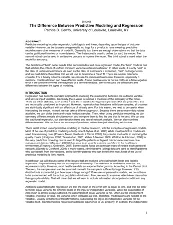
Illustrative Data: Image SegmentationIn these images, the bright green boundaries identify the cell nucleus, whilethe blue boundaries define the cell perimeter.Clearly some cells are well–segmented, meaning that they have an accurateassessment of the location and size of the cell. Others are poorlysegmented.If cell size, shape, and/or quantity are the endpoints of interest in a study,then it is important that the instrument and imaging software cancorrectly segment cells.Given a set of image measurements, how well can we predict which cellsare well–segmented (WS) or poorly–segmented (PS)?Max Kuhn (Pfizer)Predictive Modeling14 / 132
Illustrative Data: Image SegmentationMax Kuhn (Pfizer)Predictive Modeling15 / 132
Illustrative Data: Image SegmentationThe authors scored 2019 cells into these two bins.They used four stains to highlight the cell body, the cell nucleus, actin andtubulin (parts of the cytoskeleton).These correspond to di erent optical channels (e.g. channel 3 measuresactin filaments).The data are in the caret package.The authors designated a training set (n 1009) and a test set(n 1010).Max Kuhn (Pfizer)Predictive Modeling16 / 132
Data Splitting and Estimating Performance
Model Building StepsCommon steps during model building are:estimating model parameters (i.e. training models)determining the values of tuning parameters that cannot be directlycalculated from the datacalculating the performance of the final model that will generalize tonew dataHow do we “spend” the data to find an optimal model? We typically splitdata into training and test data sets:Training Set: these data are used to estimate model parameters andto pick the values of the complexity parameter(s) for the model.Test Set (aka validation set): these data can be used to get anindependent assessment of model efficacy. They should not be usedduring model training.Max Kuhn (Pfizer)Predictive Modeling18 / 132
Spending Our DataThe more data we spend, the better estimates we’ll get (provided the datais accurate). Given a fixed amount of data,too much spent in training won’t allow us to get a good assessmentof predictive performance. We may find a model that fits the trainingdata very well, but is not generalizable (over–fitting)too much spent in testing won’t allow us to get a good assessment ofmodel parametersStatistically, the best course of action would be to use all the data formodel building and use statistical methods to get good estimates of error.From a non–statistical perspective, many consumers of of these modelsemphasize the need for an untouched set of samples the evaluateperformance.Max Kuhn (Pfizer)Predictive Modeling19 / 132
Spending Our DataThere are a few di erent ways to do the split: simple random sampling,stratified sampling based on the outcome, by date and methods thatfocus on the distribution of the predictors.The base R function sample can be used to create a completely randomsample of the data. The caret package has a functioncreateDataPartition that conducts data splits within groups of the data.For classification, this would mean sampling within the classes as topreserve the distribution of the outcome in the training and test setsFor regression, the function determines the quartiles of the data set andsamples within those groupsThe segmentation data comes pre-split and we will use the originaltraining and test sets.Max Kuhn (Pfizer)Predictive Modeling20 / 132
Illustrative Data: Image Segmentation library(caret)data(segmentationData)# get rid of the cell identifiersegmentationData Cell - NULL training - subset(segmentationData, Case "Train")testing - subset(segmentationData, Case "Test")training Case - NULLtesting Case - NULLSince channel 1 is the cell body, AreaCh1 measures the size of the cell.Max Kuhn (Pfizer)Predictive Modeling21 / 132
Illustrative Data: Image Segmentation str(training[,1:9])'data.frame': 1009 obs. of Class: AngleCh1: AreaCh1: AvgIntenCh1: AvgIntenCh2: AvgIntenCh3: AvgIntenCh4: ConvexHullAreaRatioCh1 : ConvexHullPerimRatioCh1:9 variables:Factor w/ 2 levels "PS","WS": 1 2 1 2 1 1 1 2 2 2num 133.8 106.6 69.2 109.4 104.3 .int 819 431 298 256 258 358 158 315 246 223 .num 31.9 28 19.5 18.8 17.6 .num 207 116 102 127 125 .num 69.9 63.9 28.2 13.6 22.5 .num 164.2 106.7 31 46.8 71.2 .num 1.26 1.05 1.2 1.08 1.08 .num 0.797 0.935 0.866 0.92 0.931 . cell lev - levels(testing Class)Since channel 1 is the cell body, AreaCh1 measures the size of the cell.Max Kuhn (Pfizer)Predictive Modeling22 / 132
Estimating PerformanceLater, once you have a set of predictions, various metrics can be used toevaluate performance.For regression models:R 2 is very popular. In many complex models, the notion of the modeldegrees of freedom is difficult. Unadjusted R 2 can be used, but doesnot penalize complexity. (caret:::Rsquared, pls:::R2)the root mean square error is a common metric for understandingthe performance (caret:::RMSE, pls:::RMSEP)Spearman’s correlation may be applicable for models that are usedto rank samples (cor(x, y, method "spearman"))Of course, honest estimates of these statistics cannot be obtained bypredicting the same samples that were used to train the model.A test set and/or resampling can provide good estimates.Max Kuhn (Pfizer)Predictive Modeling23 / 132
Estimating Performance For ClassificationFor classification models:overall accuracy can be used, but this may be problematic when theclasses are not balanced.the Kappa statistic takes into account the expected error rate:O 1EEwhere O is the observed accuracy and E is the expected accuracyunder chance agreement (psych:::cohen.kappa, vcd:::Kappa, . . . )For 2–class models, Receiver Operating Characteristic (ROC)curves can be used to characterize model performance (more later)Max Kuhn (Pfizer)Predictive Modeling24 / 132
Estimating Performance For ClassificationA “ confusion matrix” is a cross–tabulation of the observed and predictedclassesR functions for confusion matrices are in the e1071 package (theclassAgreement function), the caret package (confusionMatrix), the mda(confusion) and others.ROC curve functions are found in the ROCR package (performance), theverification package (roc.area), the pROC package (roc) and others.We’ll use the confusionMatrix function and the pROC package later inthis class.Max Kuhn (Pfizer)Predictive Modeling25 / 132
Estimating Performance For ClassificationFor 2–class classification models we might also be interested in:Sensitivity: given that a result is truly an event, what is theprobability that the model will predict an event results?Specificity: given that a result is truly not an event, what is theprobability that the model will predict a negative results?(an “event” is really the event of interest)These conditional probabilities are directly related to the false positive andfalse negative rate of a method.Unconditional probabilities (the positive–predictive values andnegative–predictive values) can be computed, but require an estimate ofwhat the overall event rate is in the population of interest (aka theprevalence)Max Kuhn (Pfizer)Predictive Modeling26 / 132
Estimating Performance For ClassificationFor our example, let’s choose the event to be the poor segmentation(PS):Sensitivity # PS predicted to be PS# true PS# true WS to be WSSpecificity # true WSThe caret package has functions called sensitivity and specificityMax Kuhn (Pfizer)Predictive Modeling27 / 132
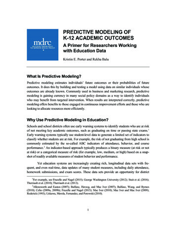
ROC CurveWith two classes the Receiver Operating Characteristic (ROC) curve canbe used to estimate performance using a combination of sensitivity andspecificity.Given the probability of an event, many alternative cuto s can beevaluated (instead of just a 50% cuto ). For each cuto , we can calculatethe sensitivity and specificity.The ROC curve plots the sensitivity (eg. true positive rate) by one minusspecificity (eg. the false positive rate).The area under the ROC curve is a common metric of performance.Max Kuhn (Pfizer)Predictive Modeling28 / 132
1.0ROC Curve From Class Probabilities 0.60.750 (0.887, 0.604)0.4 0.250 (0.588, 0.910)0.500 (0.670, 0.847)0.00.2Sensitivity0.8 1.00.80.60.40.20.0SpecificityMax Kuhn (Pfizer)Predictive Modeling29 / 132
Data Pre–Processing
Pre–Processing the DataThere are a wide variety of models in R. Some models have di erentassumptions on the predictor data and may need to be pre–processed.For example, methods that use the inverse of the predictor cross–productmatrix (i.e. (X 0 X ) 1 ) may require the elimination of collinear predictors.Others may need the predictors to be centered and/or scaled, etc.If any data processing is required, it is a good idea to base thesecalculations on the training set, then apply them to any data set used formodel building or prediction.Max Kuhn (Pfizer)Predictive Modeling31 / 132
Pre–Processing the DataExamples of of pre–processing operations:centering and scalingimputation of missing datatransformations of individual predictors (e.g. Box–Coxtransformations of the predictors)transformations of the groups of predictors, such as theIIthe “spatial–sign” transformation (i.e. x 0 x / x )feature extraction via PCA or ICAMax Kuhn (Pfizer)Predictive Modeling32 / 132
Centering, Scaling and TransformingThere are a few di erent functions for data processing in R:scale in base RScaleAdv in pcaPPstdize in plspreProcess in caretnormalize in sparseLDAThe first three functions do simple centering and scaling. preProcess cando a variety of techniques, so we’ll look at this in more detail.Max Kuhn (Pfizer)Predictive Modeling33 / 132
Centering and ScalingThe input is a matrix or data frame of predictor data. Once the values arecalculated, the predict method can be used to do the actual datatransformations.First, estimate the standardization parameters . . . trainX - training[, names(training) ! "Class"]## Methods are "BoxCox", "YeoJohnson", center", "scale",## "range", "knnImpute", "bagImpute", "pca", "ica",## "spatialSign", "medianImpute", "expoTrans"preProcValues - preProcess(trainX, method c("center", "scale"))preProcValuesCall:preProcess.default(x trainX, method c("center", "scale"))Created from 1009 samples and 58 variablesPre-processing: centered, scaledMax Kuhn (Pfizer)Predictive Modeling34 / 132
Centering and Scaling. . . then apply them to the data sets: scaledTrain - predict(preProcValues, trainX)Max Kuhn (Pfizer)Predictive Modeling35 / 132
Pre–Processing and ResamplingTo get honest estimates of performance, all data transformations shouldbe included within the cross–validation loop.The would be especially true for feature selection as well as pre–processingtechniques (e.g. imputation, PCA, etc)One function considered later called train that can apply preProcesswithin resampling loops.Max Kuhn (Pfizer)Predictive Modeling36 / 132
Over–Fitting and Resampling
Over–FittingOver–fitting occurs when a model inappropriately picks up on trends in thetraining set that do not generalize to new samples.When this occurs, assessments of the model based on the training set canshow good performance that does not reproduce in future samples.Some models have specific “knobs” to control over-fittingneighborhood size in nearest neighbor models is an examplethe number if splits in a tree modelOften, poor choices for these parameters can result in over-fittingFor example, the next slide shows a data set with two predictors. We wantto be able to produce a line (i.e. decision boundary) that di erentiates twoclasses of data.Two model fits are shown; one over–fits the training data.Max Kuhn (Pfizer)Predictive Modeling38 / 132
The DataClass 1Class 2Predictor B0.60.40.20.00.00.20.40.6Predictor AMax Kuhn (Pfizer)Predictive Modeling39 / 132
Two Model FitsClass 1Class 20.2Model #10.40.60.8Model #2Predictor B0.80.60.40.20.20.40.60.8Predictor AMax Kuhn (Pfizer)Predictive Modeling40 / 132
Characterizing Over–Fitting Using the Training SetOne obvious way to detect over–fitting is to use a test set. However,repeated “looks” at the test set can also lead to over–fittingResampling the training samples allows us to know when we are makingpoor choices for the values of these parameters (the test set is not used).Resampling methods try to “inject variation” in the system to approximatethe model’s performance on future samples.We’ll walk through several types of resampling methods for training setsamples.Max Kuhn (Pfizer)Predictive Modeling41 / 132
K –Fold Cross–ValidationHere, we randomly split the data into K distinct blocks of roughly equalsize.1We leave out the first block of data and fit a model.2This model is used to predict the held-out block3We continue this process until we’ve predicted all K held–out blocksThe final performance is based on the hold-out predictionsK is usually taken to be 5 or 10 and leave one out cross–validation haseach sample as a blockRepeated K –fold CV creates multiple versions of the folds andaggregates the results (I prefer this method)caret:::createFolds, caret:::createMultiFoldsMax Kuhn (Pfizer)Predictive Modeling42 / 132
K –Fold Cross–ValidationMax Kuhn (Pfizer)Predictive Modeling43 / 132
Repeated Training/Test Splits(aka leave–group–out cross–validation)A random proportion of data (say 80%) are used to train a model whilethe remainder is used for prediction. This process is repeated many timesand the average performance is used.These splits can also be generated using stratified sampling.With many iterations (20 to 100), this procedure has smaller variance thanK –fold CV, but is likely to be biased.caret:::createDataPartitionMax Kuhn (Pfizer)Predictive Modeling44 / 132
Repeated Training/Test SplitsMax Kuhn (Pfizer)Predictive Modeling45 / 132
BootstrappingBootstrapping takes a random sample with replacement. The randomsample is the same size as the original data set.Samples may be selected more than once and each sample has a 63.2%chance of showing up at least once.Some samples won’t be selected and these samples will be used to predictperformance.The process is repeated multiple times (say 30–100).This procedure also has low variance but non–zero bias when compared toK –fold CV.sample, caret:::createResampleMax Kuhn (Pfizer)Predictive Modeling46 / 132
BootstrappingMax Kuhn (Pfizer)Predictive Modeling47 / 132
The Big PictureWe think that resampling will give us honest estimates of futureperformance, but there is still the issue of which model to select.One algorithm to select models:Define sets of model parameter values to evaluate;for each parameter set dofor each resampling iteration doHold–out specific samples ;Fit the model on the remainder;Predict the hold–out samples;endCalculate the average performance across hold–out predictionsendDetermine the optimal parameter set;Max Kuhn (Pfizer)Predictive Modeling48 / 132
K –Nearest Neighbors ClassificationClass 1Class 2 Predictor B0.60.40.20.00.00.20.40.6Predictor AMax Kuhn (Pfizer)Predictive Modeling49 / 132
The Big Picture – K NN ExampleUsing k –nearest neighbors as an example:Randomly put samples into 10 distinct groups;for i 1 . . . 30 doCreate a bootstrap sample;Hold–out data not in sample;for k 1, 3, . . . 29 doFit the model on the boostrapped sample;Predict the i th holdout and save results;endCalculate the average accuracy across the 30 hold–out sets ofpredictionsendDetermine k based on the highest cross–validated accuracy;Max Kuhn (Pfizer)Predictive Modeling50 / 132
The Big Picture – K NN Example0.85Holdout Max Kuhn (Pfizer)Predictive Modeling51 / 132
A General StrategyThere is usually a inverse relationship between model flexibility/power andinterpretability.In the best case, we would like a parsimonious and interpretable modelthat has excellent performance.Unfortunately, that is not usually realistic.One strategy:1start with the most powerful black–box type models2get a sense of the best possible performance3then fit more simplistic/understandable models4evaluate the performance cost of using a simpler modelMax Kuhn (Pfizer)Predictive Modeling52 / 132
Training and Tuning Tree Models
Classification TreesA classification tree searches through each predictor to find a value of asingle variable that best splits the data into two groups.typically, the best split minimizes impurity of the outcome in theresulting data subsets.For the two resulting groups, the process is repeated until a hierarchicalstructure (a tree) is created.in e ect, trees partition the X space into rectangular sections thatassign a single value to samples within the rectangle.Max Kuhn (Pfizer)Predictive Modeling54 / 132
An Example First Split1TotalIntenCh2 45324Max Kuhn (Pfizer)Node 3 (n 555)PS110.80.80.60.60.40.40.20.20WSWSPSNode 2 (n 454) 45324Predictive Modeling055 / 132
The Next Round of Splitting1TotalIntenCh2 4532425IntenCoocASMCh3FiberWidthCh1 9.671Node 6 (n 154)1 9.67Node 7 (n 401)PSNode 4 (n Predictive Modeling0WS0.8WS0.8WSWSPSNode 3 (n 447) 0.6PS 0.6Max Kuhn (Pfizer) 45324056 / 132
An ExampleThere are many tree–based packages in R. The main package for fittingsingle trees are rpart, RWeka, evtree, C50 and party. rpart fits the classical“CART” models of Breiman et al (1984).To obtain a shallow tree with rpart: library(rpart) rpart1 - rpart(Class ., data training, control rpart.control(maxdepth 2)) rpart1n 1009node), split, n, loss, yval, (yprob)* denotes terminal node1) root 1009 373 PS (0.63033 0.36967)2) TotalIntenCh2 4.532e 04 454 34 PS (0.92511 0.07489)4) IntenCoocASMCh3 0.6022 447 27 PS (0.93960 0.06040) *5) IntenCoocASMCh3 0.6022 70 WS (0.00000 1.00000) *3) TotalIntenCh2 4.532e 04 555 216 WS (0.38919 0.61081)6) FiberWidthCh1 9.673 154 47 PS (0.69481 0.30519) *7) FiberWidthCh1 9.673 401 109 WS (0.27182 0.72818) *Max Kuhn (Pfizer)Predictive Modeling57 / 132
Visualizing the TreeThe rpart package has functions plot.rpart and text.rpart to visualizethe final tree.The partykit package also has enhanced plotting functions for recursivepartitioning. We can convert the rpart object to a new class called partyand plot it to see more in the terminal nodes: rpart1a - as.party(rpart1) plot(rpart1a)Max Kuhn (Pfizer)Predictive Modeling58 / 132
A Shallow rpart Tree Using the party Package1TotalIntenCh2 4532425IntenCoocASMCh3FiberWidthCh1 9.671Node 6 (n 154)1 9.67Node 7 (n 401)PSNode 4 (n Predictive Modeling0WS0.8WS0.8WSWSPSNode 3 (n 447) 0.6PS 0.6Max Kuhn (Pfizer) 45324059 / 132
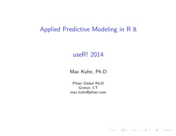
Tree Fitting ProcessSplitting would continue until some criterion for stopping is met, such asthe minimum number of observations in a nodeThe largest possible tree may over-fit and “pruning” is the process ofiteratively removing terminal nodes and watching the changes inresampling performance (usually 10–fold CV)There are many possible pruning paths: how many possible trees are therewith 6 terminal nodes?Trees can be indexed by their maximum depth and the classical CARTmethodology uses a cost-complexity parameter (Cp ) to determine besttree depthMax Kuhn (Pfizer)Predictive Modeling60 / 132
The Final TreePreviously, we told rpart to use a maximum of two splits.By default, rpart will conduct as many splits as possible, then use 10–foldcross–validation to prune the tree.Specifically, the “one SE” rule is used: estimate the standard error ofperformance for each tree size then choose the simplest tree within onestandard error of the absolute best tree size. rpartFull - rpart(Class ., data training)Max Kuhn (Pfizer)Predictive Modeling61 / 132
Tree Growing and Pruning1TotalIntenCh2 45324 4532429FiberWidthCh1 0.6 9.67 9.6710 12423AvgIntenCh1 124 323.9511SkewIntenCh1VarIntenCh4 112.3ConvexHullAreaRatioCh1 323.9 1.17 1.172431VarIntenCh4 112.3ShapeP2ACh1 172 172 1.3132632IntenCoocASMCh4KurtIntenCh3AvgIntenCh4 0.17 0.17 4.0515NeighborAvgDistCh1 218.8 4.05 375.251TotalIntenCh1 2618834AvgIntenCh4LengthCh1 218.819DiffIntenDensityCh4AvgIntenCh2 20.9336NeighborMinDistCh1 22.03 0.03 2618852ConvexHullPerimRatioCh1 20.9316 1.3 375.227AccuracyIntenCoocASMCh3 0.63AvgIntenCh2 22.033740AvgIntenCh1IntenCoocASMCh3 0.03 0.01 0.0142IntenCoocEntropyCh4 77.05 77.05 6.26 6.26 0.97 0.9743 42.09 42.09 197.8 197.8DiffIntenDensityCh4 110.7 110.7 44.41 44.4144NeighborMinDistCh1 25.64Node 30 (n 20)10.8Node 33 (n 17)10.8Node 35 (n 10)1Node 38 (n 16)10.80.8Node 39 (n 16)10.8Node 41 (n 8)10.8Node 46 (n 9)10.8 82.95Node 47 (n 15)1Node 48 (n 9)0.8Node 49 (n 26)110.80.8Node 50 (n 53)10.8Node 53 (n 17)10.8Node 54 (n 26)10.8Node 55 (n 116)1PS0.8PSNode 29 (n 11)10.8PSNode 28 (n 13)10.8PSNode 25 (n 19)1PS0.8PSNode 22 (n 15)1PS0.8PSNode 21 (n 13)1PS0.8PSNode 20 (n 12)1PS0.8PS1PSNode 18 (n 8)0.8PSNode 17 (n 21)1PS0.8PSNode 14 (n 27)1PS0.8PSNode 12 (n 58)1PS0.8PS1PS0.8PSNode 8 (n 7)1PS0.8PSNode 7 (n 7)1PSPSNode 6 (n 20WS0.60.40.20WS0.60.40.20WS0.60.4WSPS0.8PS 82.95Node 4 (n 345)1WSFull Tree 25.6445DiffIntenDensityCh40.2010 2.010 1.510 1.010 0.5cp 1 TotalIntenCh2 45324 4532425IntenCoocASMCh3 FiberWidthCh1 9.67 h1 172 0.6 1.17 172 1.31216KurtIntenCh3AvgIntenCh4 0.6 375.2Accuracy 1.1710VarIntenCh4 1.3 375.218 323.9 323.9LengthCh1 20.93 20.9320 4.05 4.05NeighborMinDistCh1 22.03 22.03 21AvgIntenCh1Node 25 (n 159)PS10.80.60.40.20WSNode 24 (n 120)PS10.80.60.40.20WSNode 23 (n 16)PS10.80.60.40.20 110.7WSNode 22 (n 16)PS10.80.60.40.20WSNode 19 (n 10)PS10.80.60.40.20WSNode 17 (n 17)PS10.80.60.40.20WSNode 14 (n 20)PS10.80.60.40.20WSNode 13 (n 24)PS10.80.60.40.20WSNode 11 (n 19)PS10.80.60.40.20WSNode 8 (n 15)PS10.80.60.40.20WSNode 7 (n 139)PS10.80.60.40.20WSNode 4 (n 7)PS10.80.60.40.20WSPSNode 3 (n 447)WSStart Pruning 110.710.80.60.40.2010 2.010 1.510 1.010 0.5cp 1 TotalIntenCh2 45324Accuracy 453243FiberWidthCh1 9.67 9.671Node 5 (n 401)PSNode 4 (n 154)PS10.80.60.60.60.40.40.40.20.20.20WS0.80 10.8WSPSWSToo Much!Node 2 (n 454) 010 2.010 1.510 1.010 0.5cpMax Kuhn (Pfizer)Predictive Modeling62 / 132
The Final Tree rpartFulln 1009node), split, n, loss, yval, (yprob)* denotes terminal node1) root 1009 373 PS (0.63033 0.36967)2) TotalIntenCh2 4.532e 04 454 34 PS (0.92511 0.07489)4) IntenCoocASMCh3 0.6022 447 27 PS (0.93960 0.06040) *5) IntenCoocASMCh3 0.6022 70 WS (0.00000 1.00000) *3) TotalIntenCh2 4.532e 04 555 216 WS (0.38919 0.61081)6) FiberWidthCh1 9.673 154 47 PS (0.69481 0.30519)12) AvgIntenCh1 323.9 139 33 PS (0.76259 0.23741) *13) AvgIntenCh1 323.9 151 WS (0.06667 0.93333) *7) FiberWidthCh1 9.673 401 109 WS (0.27182 0.72818)14) ConvexHullAreaRatioCh1 1.174 63 26 PS (0.58730 0.41270)28) VarIntenCh4 172 192 PS (0.89474 0.10526) *29) VarIntenCh4 172 44 20 WS (0.45455 0.54545)58) KurtIntenCh3 4.05 248 PS (0.66667 0.33333) *59) KurtIntenCh3 4.05 204 WS (0.20000 0.80000) *15) ConvexHullAreaRatioCh1 1.174 338 72 WS (0.21302 0.78698)30) ShapeP2ACh1 1.304 179 53 WS (0.29609 0.70391)60) AvgIntenCh4 375.2 172 PS (0.88235 0.11765) *61) AvgIntenCh4 375.2 162 38 WS (0.23457 0.76543)122) LengthCh1 20.93 103 PS (0.70000 0.30000) *123) LengthCh1 20.93 152 31 WS (0.20395 0.79605)246) NeighborMinDistCh1 22.03 32 14 WS (0.43750 0.56250)492) AvgIntenCh1 110.6 163 PS (0.81250 0.18750) *493) AvgIntenCh1 110.6 161 WS (0.06250 0.93750) *247) NeighborMinDistCh1 22.03 120 17 WS (0.14167 0.85833) *31) ShapeP2ACh1 1.304 159 19 WS (0.11950 0.88050) *Max Kuhn (Pfizer)Predictive Modeling63 / 132
The Final rpart Tree1TotalIntenCh2 45324 4532425IntenCoocASMCh3FiberWidthCh1 9.67 9.6769AvgIntenCh1ConvexHullAreaRatioCh1 1.1715VarInten
Applied Predictive Modeling in R R useR! 2014 Max Kuhn, Ph.D Pfizer Global R&D Groton, CT max.kuhn@pfizer.com. Outline Conventions in R Data Splitting and Estimating Performance Data Pre-Processing Over–Fitting and Resampling Training and Tuning