Transcription
Extending Steinberg’s Fatigue Analysis of Electronics Equipment Methodologyto a Full Relative Displacement vs. Cycles CurveRevision CBy Tom IrvineEmail: tom@vibrationdata.comMarch 13, 2013Vibration fatigue calculations are “ballpark” calculations given uncertainties in S-N curves,stress concentration factors, natural frequency, damping and other variables. Furthermore,damage increases exponentially with an increase in stress, which magnifies the effect of anyerror in the stress calculation or in the reference S-N curve. Perhaps the best that can beexpected is to calculate the accumulated fatigue to the correct “order-of-magnitude.”IntroductionElectronic components in vehicles are subjected to shock and vibration environments. Thecomponents must be designed and tested accordingly. Dave S. Steinberg’s Vibration Analysisfor Electronic Equipment is a widely used reference in the aerospace and automotive industries.Steinberg’s text gives practical empirical formulas for determining the fatigue limits forelectronics piece parts mounted on circuit boards. The concern is the bending stress experiencedby solder joints and lead wires.The fatigue limits are given in terms of the maximum allowable 3-sigma relative displacement ofthe circuit boards for the case of 20 million stress reversal cycles at the circuit board’s naturalfrequency. The vibration is assumed to be steady-state with a Gaussian distribution.Note that classical fatigue methods use stress as the response metric of interest. But Steinberg’sapproach works in an approximate, empirical sense because the bending stress is proportional tostrain, which is in turn proportional to relative displacement.The user then calculates the expected 3-sigma relative displacement for the component ofinterest and then compares this displacement to the Steinberg limit value.There are several limitations to Steinberg’s fatigue limit method:1. An electronic component’s service life may be well below or well above 20million cycles.1
2. A component may undergo nonstationary or non-Gaussian random vibrationsuch that its expected 3-sigma relative displacement does not adequatelycharacterize its response to its service environments.3. The component’s circuit board will likely behave as a multi-degree-offreedom system, with higher modes contributing non-negligible bendingstress, and in such a manner that the stress reversal cycle rate is greater thanthat of the fundamental frequency alone.These obstacles can be overcome by developing a “relative displacement vs. cycles” curve,similar to an S-N curve.Fortunately, Steinberg has provides the pieces for constructing this RD-N curve, with “someassembly required.” Note that RD is relative displacement.The analysis can then be completed using the rainflow cycle counting for the relativedisplacement response and Miner’s accumulated fatigue equation.Steinberg’s Fatigue Limit EquationLhRelative MotionComponentZBRelative MotionComponentComponentFigure 1. Component and Lead Wires undergoing Bending Motion2
Let Z be the single-amplitude displacement at the center of the board that will give a fatigue lifeof about 20 million stress reversals in a random-vibration environment, based upon the 3 circuitboard relative displacement.Steinberg’s empirical formula for Z 3 limit isZ 3 limit 0.00022 BCh rLinches(1)whereB length of the circuit board edge parallel to the component, inchesL length of the electronic component, inchesh circuit board thickness, inchesr relative position factor for the component mounted on the board(Table 1)C Constant for different types of electronic components (Table 2)0.75 C 2.25Equation (1) is taken from Reference 1.Table 1. Relative Position Factors for Component on Circuit BoardrComponent Location(Board supported on all sides)1When component is at center of PCB(half point X and Y).0.707When component is at half point X and quarter point Y.0.50When component is at quarter point X and quarter pointY.3
Table 2. Constant for Different Types of Electronic ComponentsC0.75ComponentAxial leaded through holeor surface mountedcomponents, resistors,capacitors, diodes1.0Standard dual inlinepackage (DIP)1.26DIP with side-brazed leadwiresImage4
Table 2. Constant for Different Types of Electronic Components (continued)C1.0ComponentThrough-hole Pin grid array(PGA) with many wiresextending from the bottomsurface of the PGA2.25Surface-mounted leadlessceramic chip carrier(LCCC).ImageA hermetically sealedceramic package. Instead ofmetal prongs, LCCCs havemetallic semicircles (calledcastellations) on their edgesthat solder to the pads.1.26Surface-mounted leadedceramic chip carriers withthermal compressionbonded J wires or gull wingwires.5
Table 2. Constant for Different Types of Electronic Components (continued)C1.75ComponentSurface-mounted ball grid array(BGA).ImageBGA is a surface mount chipcarrier that connects to a printedcircuit board through a bottomside array of solder balls.0.751.26Fine-pitch surface mountedaxial leads around perimeter ofcomponent with four cornersbonded to the circuit board toprevent bouncingAny component with twoparallel rows of wires extendingfrom the bottom surface,hybrid, PGA, very large scaleintegrated (VLSI), applicationspecific integrated circuit(ASIC), very high scaleintegrated circuit (VHSIC), andmultichip module (MCM).6
Sample Base Input PSDAn RD-N curve will be constructed for a particular case. The resulting curve can then berecalibrated for other cases.Consider a circuit board which behaves as a single-degree-of-freedom system, with a naturalfrequency of 500 Hz and Q 10. These values are chosen for convenience but are somewhatarbitrary.The system is subjected to the base input shown in Table 3.Table 3. Base Input PSD, 8.8 GRMSFrequency (Hz)Accel (G 2/Hz)200.00531500.0420000.04The duration will be 1260 seconds, but the response results will be extended as a “test to failure.”Note that accumulated fatigue damage for random vibration response increases approximatelylinearly with increase in duration. The relationship may have some nonlinearity due to therandom occurrence of response peaks above 3-sigma.Time History SynthesisThe next step is to generate a time history that satisfies the base input PSD in Table 3.The synthesis is performed using the method in Reference 2. The total 1260-second duration isrepresented as three consecutive 420-second segments. Separate segments are calculated due tocomputer processing speed and memory limitations.The complete time history set is shown in Figure 2.Each segment essentially has a Gaussian distribution, but the histogram plots are also omitted forbrevity. The actual histograms have a slight deviation from the Gaussian ideal due to the effectof the fade in, but this is incidental.Verification that the complete time history satisfies the PSD specification is shown in Figure 3.7
SYNTHESIZED TIME HISTORY No. 18.8 GRMS OVERALL60ACCEL (G)40200-20-40-60050100150200250300350400TIME (SEC)SYNTHESIZED TIME HISTORY No. 28.8 GRMS OVERALL60ACCEL (G)40200-20-40-60050100150200250300350400TIME (SEC)SYNTHESIZED TIME HISTORY No. 38.8 GRMS OVERALL60ACCEL (G)40200-20-40-60050100150200250300350400TIME (SEC)Figure 2.8
POWER SPECTRAL DENSITY1Time History 3Time History 2Time History 1Specification2ACCEL (G /Hz)0.10.010.0012010010002000FREQUENCY (Hz)Figure 3.Each curve has an overall level of 8.8 GRMS. The curves are nearly identical.SDOF ResponseThe response analysis is performed using the ramp invariant digital recursive filteringrelationship in Reference 3.The response results are shown in Figure 4. Descriptive statistics are shown in Table 4.9
RELATIVE DISPLACEMENT RESPONSE No. 1fn 500 Hz Q 10REL DISP 00250300350400TIME (SEC)RELATIVE DISPLACEMENT RESPONSE No. 2fn 500 Hz Q 10REL DISP 00250300350400TIME (SEC)RELATIVE DISPLACEMENT RESPONSE No. 3fn 500 Hz Q 10REL DISP 00250300350400TIME (SEC)Figure 4.10
Table 4. Relative Displacement Response 420.0006830.00068No.KurtosisCrest Factor3.025.110.002043.035.440.002043.015.25Note that the crest factor is the ratio of the peak-to-standard deviation, or peak-to-rms assumingzero mean.Kurtosis is a parameter that describes the shape of a random variable’s histogram or itsequivalent probability density function (PDF).Rainflow Cycle CountingTable 5.Relative Displacement Results from Rainflow Cycle Counting, Bin Format, Unit: inch, 1260-sec .50.00000.00010.000-0.00260.00280.00000.000211
Next, a rainflow cycle count was performed on the relative displacement time histories using themethod in Reference 4. The combined, binned results are shown in Table 5. Note that:Amplitude (peak-valley)/2.The total number of cycles was 698903. This corresponds to a rate of 555 cycles/sec over the1260 second duration. This rate is about 10% higher than the 500 Hz natural frequency.The binned results are shown mainly for reference, given that this is a common presentationformat in the aerospace industry. The binned results could be inserted into a Miner’s cumulativefatigue calculation.The method in this analysis, however, will use the raw rainflow results consisting of cycle-bycycle amplitude levels, including half-cycles. This brute-force method is more precise thanusing binned data.Also, note that rainflow counting can be performed more quickly using a C program ratherthan a Matlab script, in the author’s experience. This is especially true if the time history hasmillions of data points.Miner’s Accumulated FatigueLet n be the number of stress cycles accumulated during the vibration testing at a given levelstress level represented by index i.Let N be the number of cycles to produce a fatigue failure at the stress level limit for thecorresponding index.Miner’s cumulative damage index CDI is given bym niCDI Ni 1 i (2)where m is the total number of cycles or bins depending on the analysis type.In theory, the part should fail whenCDI 1.0(3)Miner’s index can be modified so that it is referenced to relative displacement rather than stress.Note that the zero-to-peak form of relative displacement will be used throughout the remainderof this paper.12
Derivation of the RD-N CurveThe exponent b is taken as 6.4 for PCB-component lead wires. This number is derived in Reference 1,section 7.3, page 177. It represents generic metal. It is used in Reference 1 for both sine and randomvibration.The goal is to determine an RD-N curve of the formlog10 (N) -6.4 log10 (RD) a(4)whereNRDais the number of cyclesrelative displacement (inch)unknown variableThe unknown variable will be determined by calibration.a log10 (N) 6.4 log10 (RD)(5)Let N 20 million reversal cycles.a 7.30 6.4 log10 (RD)(6)Now assume that the process in the preceding example was such that its 3-sigma relativedisplacement reached the limit in equation (1) for 20 million cycles. This would require that theduration 1260 second duration be multiplied by 28.6.28.6 (20 million cycles-to-failure )/( 698903 rainflow cycles )Now apply the RD-N equation (4) along with Miner’s equation (2) to the rainflow cycle-by-cycleamplitude levels with trial-and-error values for the unknown variable a. Multiply the CDI by the28.6 scale factor to reach 20 million cycles. Iterate until a value of a is found such that CDI 1.0.13
The numerical experiment result isa -11.20for a 3-sigma limit of 0.00204 inchThe 3-sigma value matches that in Table 4.Substitute into equation (4).log10 (N) -6.4 log10 (RD) -11.20for a 3-sigma limit of 0.00204 inch(7)Equation (7) will be used for the “high cycle fatigue” portion of the RD-N curve. A separatecurve will be used for “low cycle fatigue.”The low cycle portion will be based on another Steinberg equation that the maximum allowablerelative displacement for shock is six times the 3-sigma limit value at 20 million cycles forrandom vibration.But the next step is to derive an equation for a as a function of 3-sigma limit without resorting tonumerical experimentation.LetRDx RD at N 20 million. a - 7.30 RDx 10 6.4 RDx 0.0013 inch for a -11.20a 7.3 6.4 log10 (0.0013) -11.20 for a 3-sigma limit of 0.00204 inch(8)(9)(10)The RDx value is not the same as the Z 3 limit .But RDx should be directly proportional to Z 3 limit .14
So postulate thata 7.3 6.4 log10 (0.0026) -9.24 for a 3-sigma limit of 0.00408 inch(11)This was verified by experiment where the preceding time histories were doubled and CDI 1.0was achieved after the rainflow counting.Thus, the following relation is obtained.Z 3 limit a 7.3 6.4 log10 (0.0013) 0.00204 inch a 7.3 6.4 log10 (0.637) Z 3 limit(12) (13) log10 (N) -6.4 log10 (RD) 7.3 6.4 log10 (0.637) Z 3 limit log10 (N) 7.3 - 6.4 log10 (0.637) Z 3 limit log10 (RD) RDlog10 (N) 7.3 - 6.4 log10 0.637 Z 3 limit RD log10 (N) 6.05 - 6.4 log10 Z 3 limit (14)(15)(16)(17)The final RD-N equation for high-cycle fatigue is RD 6.05 - log10 (N)log10 6.4 Z 3 limit (18)15
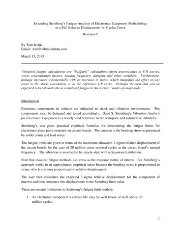
RD-N CURVEELECTRONIC COMPONENTSRD / Z 3- limit1010.1010101102103104105106107108CYCLESFigure 5.Equation (18) is plotted in Figure 5 along with the low-cycle fatigue limit.RD is the zero-to-peak relative displacement.Again, the low cycle portion is based on another Steinberg equation that the maximum allowablerelative displacement ratio for shock is six times the 3-sigma limit value at 20 million cycles forrandom vibration. The physical explanation is that a “strain hardening effect” occurs at therelative displacement ratio corresponding to the plateau region below 200 cycles.In reality, transition between the plateau and the downward ramp would be a smooth curve. Thisis a topic for future research.16
Sine and Random Damage EquivalenceContinue with the previous example for the case where there were 20 million cycles andCDI 1.0.This is also the special case where the 3-sigma relative displacement equalsSteinberg’s Z 3 limit .Note that RD 0.64 Z 3 limit at 20 million cycles(19)Again, RD and Z 3 limit are different parameters which have a common length dimension.RD is the zero-to-peak relative displacement, which varies cycle-by-cycle.Z 3 limit is the 3-sigma relative displacement limit from Steinberg. Note that 1.1l% of the absoluteresponse peaks are greater than 3-sigma for the case where the response peaks have a Rayleighdistribution.Any individual point along the RD-N curve must be considered in terms of an “equivalent sine”oscillation.Again the relative displacement ratio at 20 million cycles is 0.64.(0.64)(3-sigma) 1.9-sigma(20)This suggests that “damage equivalence” between sine and random vibration occurs when theresponse sine amplitude (zero-to-peak) is approximately equal to the random vibration 2-sigmaamplitude. This relationship was previously derived in Reference 5. The base input sineamplitude would then be the response sine amplitude divided by the Q factor.Please also refer to the example in Appendix A which gives experimental verification of theequivalent sine for a case where CDI 1 and the total cycle number is 20 million.17
ExamplesExamples for particular piece parts are given in Appendices A through C.ConclusionA methodology for developing RD-N curves for electronic components was presented in thispaper. The method is an extrapolation of the empirical data and equations given in Steinberg’stext.The method is particularly useful for the case where a component must undergo nonstationaryvibration, or perhaps a series of successive piecewise stationary base input PSDs.The resulting RD-N curve should be applicable to nearly any type of vibration, includingrandom, sine, sine sweep, sine-or-random, shock, etc.It is also useful for the case where a circuit board behaves as a multi-degree-of-freedom system.This paper also showed in a very roundabout way that “damage equivalence” between sine andrandom vibration occurs when the sine amplitude (zero-to-peak) is approximately equal to therandom vibration 2-sigma amplitude.This remains a “work-in-progress.” Further investigation and research is needed.References1. Dave S. Steinberg, Vibration Analysis for Electronic Equipment, Second Edition, WileyInterscience, New York, 1988.2. T. Irvine, A Method for Power Spectral Density Synthesis, Rev B, Vibrationdata, 2000.3. David O. Smallwood, An Improved Recursive Formula for Calculating Shock ResponseSpectra, Shock and Vibration Bulletin, No. 51, May 1981.4. ASTM E 1049-85 (2005) Rainflow Counting Method, 1987.5. T. Irvine, Sine and Random Vibration Equivalent Damage, Revision A, Vibrationdata, 2004.6. T. Irvine, Plate Bending Frequencies via the Finite Element Method with RectangularElements, Revision A, 2011.7. T. Irvine, Modal Transient Analysis of a Multi-degree-of-freedom System with EnforcedMotion, Revision C, Vibrationdata, 2011.18
APPENDIX ASingle-degree-of-freedom, Stationary Vibration ExampleConsider a Ball Grid Array (BGA) mounted at the center of an electronics board.parameters are given in Table A-1.TheAssume that the circuit board behaves as a single-degree-of-freedom system with a naturalfrequency of 400 Hz and Q 10.Table A-1. Example ParametersB 6.0 inchCircuit board lengthL 1.0 inchPart lengthh 0.093 inchr 1.0Center of circuit board from Table 1C 1.75BGA component from Table 2fn 400 HzCircuit board natural frequencyQ 10Circuit board thicknessAmplification factor19
Calculate the relative displacement limit.Z 3 limit 0.00022 BCh r LZ 3 limit inches0.00022 6.0 1.75 0.093 1.0 Z 3 limit 0.00811.0(A-1)inches(A-2)inches(A-3)Now consider that the circuit board is subjected to the base input in Table 1 plus 12 dB.input level is thus 35.2 GRMS overall.TheThe synthesized time histories from Figure 4 are raised by 12 dB are used as a base input.The relative displacement response is calculated via Reference 3. The levels are shown in TableA-2.Table A-2. Relative Displacement Response 0.003830.0038No.KurtosisCrest Factor3.044.810.01143.045.250.01143.025.05The rainflow cycle counting is performed using Reference 4.The CDI is calculated using the curve in Figure 5.The result is: CDI 0.242 for 1260 seconds and 12 dB marginThe number of rainflow cycles was 574,680. The rainflow cycle rate was 456 Hz.20
Equivalent SineConsider a 400 Hz sine function over 1260 seconds. The total number of cycles is 504,000.Derive the sine amplitude so the resulting CDI is the same as that for the random vibration case.Now divide the actual cycle number by the CDI.( 504,000 cycles) / (0.242) 2,082,644 cycles(A-4)Thus 2,082,644 cycles would have been allowed for the yet-to-be-determined relativedisplacement amplitude.Note that from the RD-N curve RD 0.908 Z 3 limit at 2,082,644 cyclesRD 0.908 Z 3 limit(A-5)(A-6)Again, for this example,Z 3 limit 0.0081inches(A-7)Now calculate the equivalent sine amplitude with respect to this limit.RD 0.908 0.0081 inches (A-8)RD 0.0074 inches(A-9)21
Now divide the equivalent sine amplitude by the random vibration relative displacement responsestandard deviation from Table A-2.( 0.0074 inches / 0.0038 inches ) 1.9(A-10)Thus, an “equivalent sine” would be approximately 2-sigma in terms of the respective sine andrandom relative displacement response amplitudes.Time-to FailureAgain, damage is approximately linearly proportional to duration. .Thus, by extrapolation: CDI 1.0 for 5204 seconds and 12 dB marginThe time-to-failure is thus about 87 minutes.22
APPENDIX BSingle-degree-of-freedom, Nonstationary VibrationReconsider the Ball Grid Array mounted at the center of an electronics board from Appendix A.Change the board natural frequency to 450 Hz. All other material and geometry parametersremain the same.Again,Z 3 limit 0.0081inches(B-1)The part is subjected to the flight accelerometer data shown as in Figure B-1.corresponding Waterfall FFT is given in Figure B-2.TheThis is a sine sweep driven by a “resonant burn” effect in the solid rocket motor combustionchamber. It is nonstationary. The duration is about 20 seconds.FLIGHT ACCELEROMETER DATA SOLID ROCKET MOTOR BURNMotor Adapter Bulkhead Longitudinal Axis32ACCEL (G)10-1-2-3424446485052545658606264TIME (SEC)Figure B-1.23
Waterfall FFT Solid Rocket Motor OscillationFlight Accelerometer Data Motor Adapter Bulkhead Longitudinal AxisMagnitudeTime (sec)Frequency (Hz)Figure B-2.The overall response relative displacement is 0.00018 inches for the zero margin case.The rainflow cycle counting is performed using Reference 4.The CDI is calculated using the curve in Figure 6.The result is:CDI 3.64e-11for 20 seconds and zero marginCDI 3.03e-09for 20 seconds and 6 dB marginThe CDI is negligibly low for each margin.24
But assume the component had been subject to a random vibration test, but not a sine sweep test,before the flight.A CDI could be calculated for the random vibration test in order to determine whether it coveredthe flight sine sweep in terms of fatigue.25
APPENDIX CMulti-degree-of-freedom, Stationary Vibration ExampleConsider a Ball Grid Array (BGA) mounted on electronics board. The parameters are given inTable C-1.Table C-1. Example ParametersB 3.0 x 6.0 inch Circuit board length & widthL 0.5 inchh 0.093 inchr 1.0Center of Board from Table 1C 1.75BGA component from Table 2Q 10Part lengthCircuit board thicknessAmplification factor for all modesThe board boundary conditions are shown in Figure C-1.freefixedfixed6 infixed3 inFigure C-1.26
Calculate the relative displacement limit.Set B 3.0 inch, the width, for conservatism. Note that the BGA in this example is square.Z 3 limit Z 3 limit 0.00022 BCh r Linches0.00022 3.0 1.75 0.093 1.0 Z 3 limit 0.00570.5(C-1)inchesinches(C-2)(C-3)Also assume that the total board mass is 0.31 lbm with a uniform distribution.The finite element method is used to calculate the circuit board response via Reference 5.The first four natural frequencies of the board arenfn(Hz)181829373121041667The relative displacement transmissibility for the center of the board is shown in Figure C-2.27
Figure C-2.Note that the largest peak represents the combined response of the 818 and 937 Hz modesNow consider that the circuit board is subjected to the base input in Table 1 plus 12 dB.Determine the time-to-failure.The first (top) synthesized time history from Figure 4 is used as a base input. Only the first 150seconds of this record is used due to the author’s computer memory limitations. The fullduration will be used in the next revision of this paper. Pushing large time histories throughmulti-degree-of-freedom finite element models for modal transient analysis is a challenge.The response for the 150-second duration is calculated via Reference 6.The rainflow cycle counting is performed using Reference 4.28
The CDI is calculated using the curve in Figure 5.The result is:CDI 0.000338for 150 seconds and 12 dB marginAgain, damage is approximately linearly proportional to duration.Failure would occur at about 123 hours for the 12 dB margin case.Note the relative displacement tends to be higher for lower natural frequency components. Inthis case, the first two natural frequencies were 818 and 937 Hz, which were sufficiently high fora relatively long life at the elevated level.29
Electronic components in vehicles are subjected to shock and vibration environments. The components must be designed and tested accordingly. Dave S. Steinberg’s Vibration Analysis for Electronic Equipment is a widely u