Transcription
Excel ChartsAbout the TutorialA chart is a tool you can use in Excel to communicate data graphically. Charts allow youraudiencetoseethe meaningbehindthenumbers,andtheymakeshowing comparisons and trends much easier. In this tutorial, you will learn how toinsert charts and modify them so they communicate information effectively.Each of Excel's 12 chart types has different features that make them better suited forspecific tasks. Pairing a chart with its correct data style will make the information easierto understand, enhancing the communication within your small business.AudienceGraphs or charts help people understand data quickly. Whether you want to make acomparison, show a relationship or highlight a trend, they help your audience “see” whatyou are talking about.Among its many features, Microsoft Excel enables you to incorporate charts, providing away to add visual appeal to your business reports.PrerequisitesBefore you start proceeding with this tutorial, we are assuming that you are already awareof the basics of Microsoft Excel. If you are not well aware of these concepts, then we willsuggest you to go through our short tutorials on Excel.Copyright & Disclaimer Copyright 2018 by Tutorials Point (I) Pvt. Ltd.All the content and graphics published in this e-book are the property of Tutorials Point (I)Pvt. Ltd. The user of this e-book is prohibited to reuse, retain, copy, distribute or republishany contents or a part of contents of this e-book in any manner without written consentof the publisher.We strive to update the contents of our website and tutorials as timely and as precisely aspossible, however, the contents may contain inaccuracies or errors. Tutorials Point (I) Pvt.Ltd. provides no guarantee regarding the accuracy, timeliness or completeness of ourwebsite or its contents including this tutorial. If you discover any errors on our website orin this tutorial, please notify us at contact@tutorialspoint.comi
Excel ChartsTable of ContentsAbout the Tutorial . iAudience . iPrerequisites . iCopyright & Disclaimer . iTable of Contents . ii1.Excel Charts – Introduction . 1Charts Group . 1Chart Tools. 2Recommended Charts . 22.Excel Charts – Creating Charts . 4Creating Charts with Insert Chart . 4Creating Charts with Recommended Charts . 6Creating Charts with Quick Analysis . 93.Excel Chart – Types . 13Column Chart . 13Line Chart . 14Pie Chart . 14Doughnut Chart . 14Bar Chart . 14Area Chart. 15XY (Scatter) Chart . 15Bubble Chart . 16Stock Chart . 16Surface Chart . 17Radar Chart . 17Combo Chart. 174.Excel Charts – Column Chart . 18Clustered Column and 3-D Clustered Column . 20Stacked Column and 3-D Stacked Column . 21100% Stacked Column and 3-D 100% Stacked Column . 213-D Column . 225.Excel Charts – Line Chart . 23Line and Line with Markers . 25Stacked Line and Stacked Line with Markers . 26100% Stacked Line and 100% Stacked Line with Markers . 273-D Line . 286.Excel Charts – Pie Chart . 29Pie and 3-D Pie. 31Pie of Pie and Bar of Pie . 327.Excel Charts – Doughnut Chart . 348.Excel Charts – Bar Chart . 37ii
Excel ChartsClustered Bar and 3-D Clustered Bar . 39Stacked Bar and 3-D Stacked Bar. 40100% Stacked Bar and 3-D 100% Stacked Bar . 419.Excel Charts – Area Chart . 42Area and 3-D Area . 44Stacked Area and 3-D Stacked Area . 45100% Stacked Area and 3-D 100% Stacked Area . 4610. Excel Charts – Scatter (X Y) Chart . 47Scatter Chart . 50Types of Scatter Charts . 5011. Excel Charts – Bubble Chart . 53Bubble and 3-D Bubble . 5512. Excel Charts – Stock Chart . 56High-Low-Close . 58Open-High-Low-Close . 58Volume-High-Low-Close . 59Volume-Open-High-Low-Close . 6013. Excel Charts – Surface Chart . 613-D Surface . 63Wireframe 3-D Surface . 64Contour. 65Wireframe Contour . 6614. Excel Charts – Radar Chart . 67Radar and Radar with Markers . 69Filled Radar . 6915. Excel Charts – Combo Charts . 70Clustered Column – Line . 72Clustered Column – Line on Secondary Axis . 72Stacked Area – Clustered Column . 73Custom Combo Chart . 7416. Excel Charts – Chart Elements . 76Axes . 79Axis Titles . 80Chart Title . 83Data Labels . 85Data Table. 87Error Bars . 88Gridlines . 90Legend . 92Trendline . 9317. Excel Charts – Chart Styles . 94Style . 94Color . 96iii
Excel Charts18. Excel Charts – Chart Filters . 101Values . 102Names . 10419. Excel Charts – Fine Tuning . 108Format Style . 110Format Color . 111Chart Filters . 11220. Excel Charts – Design Tools . 114Add Chart Element . 115Quick Layout . 116Change Colors . 117Chart Styles . 118Switch Row/Column . 118Select Data . 119Change Chart Type . 121Move Chart . 12221. Excel Charts – Quick Formatting . 123Format Pane . 123Format Axis . 126Format Chart Title . 128Format Chart Area . 128Format Plot Area . 129Format Data Series . 129Format Data Labels . 130Format Data Point . 131Format Legend. 132Format Major Gridlines . 13222. Excel Charts – Aesthetic Data Labels . 133Data Label Positions . 134Format a Single Data Label . 135Data Labels with Effects . 137Shape of a Data Label . 139Resize a Data Label . 140Add a Field to a Data Label . 141Connecting Data Labels to Data Points . 144Format Leader Lines . 14523. Excel Charts – Format Tools . 146Current Selection Group . 148Insert Shapes Group . 149Shape Styles Group . 149WordArt Styles Group . 150Arrange Group . 151Size Group . 15224. Excel Charts – Sparklines . 153Sparklines with Quick Analysis . 153Sparklines with INSERT tab . 157iv
Excel Charts25. Excel Charts – PivotChart . 164Creating a PivotChart from a PivotTable . 164Recommended Pivot Charts . 170v
1. Excel Charts – IntroductionExcel ChartsIn Microsoft Excel, charts are used to make a graphical representation of any set of data. Achart is a visual representation of data, in which the data is represented by symbols suchas bars in a bar chart or lines in a line chart.Charts GroupYou can find the Charts group under the INSERT tab on the Ribbon.The Charts group on the Ribbon looks as follows-The Charts group is formatted in such a way that Types of charts are displayed. The subgroups are clubbed together. It helps you find a chart suitable to your data with the button Recommended Charts.1
Excel ChartsChart ToolsWhen you click on a chart, a new tab Chart Tools is displayed on the ribbon. There are twotabs under CHART TOOLS DESIGN FORMATRecommended ChartsThe Recommended Charts command on the Insert tab helps you to create a chart that isjust right for your data.2
Excel ChartsTo use Recommended chartsStep 1: Select the data.Step 2: Click Recommended Charts.A window displaying the charts that suit your data will be displayed.3
2. Excel Charts – Creating ChartsExcel ChartsIn this chapter, we will learn to create charts.Creating Charts with Insert ChartTo create charts using the Insert Chart tab, follow the steps given below.Step 1: Select the data.Step 2: Click the Insert tab on the Ribbon.Step 3: Click the Insert Column Chart on the Ribbon.4
Excel ChartsThe 2-D column, 3-D Column chart options are displayed. Further, More Column Charts option is also displayed.Step 4: Move through the Column Chart options to see the previews.Step 5: Click Clustered Column. The chart will be displayed in your worksheet.5
Excel ChartsStep 6: Give a meaningful title to the chart by editing Chart Title.Creating Charts with Recommended ChartsYou can use the Recommended Charts option if You want to create a chart quickly. You are not sure of the chart type that suits your data. If the chart type you selected is not working with your data.To use the option Recommended Charts, follow the steps given belowStep 1: Select the data.Step 2: Click the Insert tab on the Ribbon.Step 3: Click Recommended Charts.A window displaying the charts that suit your data will be displayed, under the tabRecommended Charts.6
Excel ChartsStep 4: Browse through the Recommended Charts.Step 5: Click on a chart type to see the preview on the right side.7
Excel ChartsStep 6: Select the chart type you like. Click OK. The chart will be displayed in yourworksheet.If you do not see a chart you like, click the All Charts tab to see all the available charttypes and pick a chart.Step 7: Give a meaningful title to the chart by editing Chart Title.8
Excel ChartsCreating Charts with Quick AnalysisFollow the steps given to create a chart with Quick Analysis.Step 1: Select the data.A Quick Analysis buttonappears at the bottom right of your selected data.Step 2: Click the Quick Analysisicon.The Quick Analysis toolbar appears with the options FORMATTING, CHARTS, TOTALS,TABLES, SPARKLINES.9
Excel ChartsStep 3: Click the CHARTS option.Recommended Charts for your data will be displayed.Step 4: Point the mouse over the Recommended Charts. Previews of the availablecharts will be shown.10
Excel ChartsStep 5: Click More.More Recommended Charts will be displayed.11
Excel ChartsStep 6: Select the type of chart you like, click OK. The chart will be displayed in yourworksheet.Step 7: Give a meaningful title to the chart by editing Chart Title.12
3. Excel Chart – TypesExcel ChartsExcel provides you different types of charts that suit your purpose. Based on the type ofdata, you can create a chart. You can also change the chart type later.Excel offers the following major chart types Column Chart Line Chart Pie Chart Doughnut Chart Bar Chart Area Chart XY (Scatter) Chart Bubble Chart Stock Chart Surface Chart Radar Chart Combo ChartEach of these chart types have sub-types. In this chapter, you will have an overview ofthe different chart types and get to know the sub-types for each chart type.Column ChartA Column Chart typically displays the categories along the horizontal (category) axis andvalues along the vertical (value) axis. To create a column chart, arrange the data incolumns or rows on the worksheet.A column chart has the following sub-types Clustered Column. Stacked Column. 100% Stacked Column. 3-D Clustered Column. 3-D Stacked Column. 3-D 100% Stacked Column. 3-D Column.13
Excel ChartsLine ChartLine charts can show continuous data over time on an evenly scaled Axis. Therefore, theyare ideal for showing trends in data at equal intervals, such as months, quarters or years.In a Line chart Category data is distributed evenly along the horizontal axis. Value data is distributed evenly along the vertical axis.To create a Line chart, arrange the data in columns or rows on the worksheet.A Line chart has the following sub-types: Line Stacked Line 100% Stacked Line Line with Markers Stacked Line with Markers 100% Stacked Line with Markers 3-D LinePie ChartPie charts show the size of items in one data series, proportional to the sum of the items.The data points in a pie chart are shown as a percentage of the whole pie. To create a PieChart, arrange the data in one column or row on the worksheet.A Pie Chart has the following sub-types Pie 3-D Pie Pie of Pie Bar of PieDoughnut ChartA Doughnut chart shows the relationship of parts to a whole. It is similar to a Pie Chartwith the only difference that a Doughnut Chart can contain more than one data series,whereas, a Pie Chart can contain only one data series.A Doughnut Chart contains rings and each ring representing one data series. To create aDoughnut Chart, arrange the data in columns or rows on a worksheet.Bar ChartBar Charts illustrate comparisons among individual items. In a Bar Chart, the categoriesare organized along the vertical axis and the values are organized along the horizontalaxis. To create a Bar Chart, arrange the data in columns or rows on the Worksheet.14
Excel ChartsA Bar Chart has the following sub-types Clustered Bar Stacked Bar 100% Stacked Bar 3-D Clustered Bar 3-D Stacked Bar 3-D 100% Stacked BarArea ChartArea Charts can be used to plot the change over time and draw attention to the total valueacross a trend. By showing the sum of the plotted values, an area chart also shows therelationship of parts to a whole. To create an Area Chart, arrange the data in columns orrows on the worksheet.An Area Chart has the following sub-types Area Stacked Area 100% Stacked Area 3-D Area 3-D Stacked Area 3-D 100% Stacked AreaXY (Scatter) ChartXY (Scatter) charts are typically used for showing and comparing numeric values, likescientific, statistical, and engineering data.A Scatter chart has two Value Axes Horizontal (x) Value Axis Vertical (y) Value AxisIt combines x and y values into single data points and displays them in irregular intervals,or clusters. To create a Scatter chart, arrange the data in columns and rows on theworksheet.Place the x values in one row or column, and then enter the corresponding y values in theadjacent rows or columns.Consider using a Scatter chart when You want to change the scale of the horizontal axis. You want to
Excel Charts 1 In Microsoft Excel, charts are used to make a graphical representation of any set of data. A chart is a visual representation of data, in which the data is represented by symbols such as bars in a bar chart or lines in a line chart. Charts Group You can