Transcription
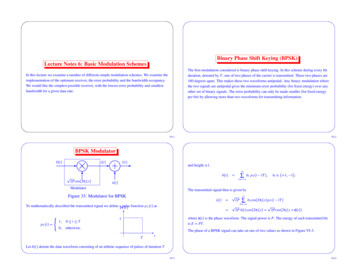
Binary Phase Shift Keying (BPSK)Lecture Notes 6: Basic Modulation SchemesThe first modulation considered is binary phase shift keying. In this scheme during every bitduration, denoted by T , one of two phases of the carrier is transmitted. These two phases are180 degrees apart. This makes these two waveforms antipodal. Any binary modulation wherethe two signals are antipodal gives the minimum error probability (for fixed energy) over anyother set of binary signals. The error probability can only be made smaller (for fixed energyper bit) by allowing more than two waveforms for transmitting information.In this lecture we examine a number of different simple modulation schemes. We examine theimplementation of the optimum receiver, the error probability and the bandwidth occupancy.We would like the simplest possible receiver, with the lowest error probability and smallestbandwidth for a given data rate. VI-1strtand height 1. bl pT tlTbl11 l "! bt 2P cos 2π f ct bt BPSK ModulatorVI-2 nt ModulatorThe transmitted signal then is given by Figure 33: Modulator for BPSK tT0otherwise.lT2P cos 2π f ctφt 0bl cos 2π f ct pT twhere φ t is the phase waveform. The signal power is P. The energy of each transmitted bitis E PT .1 1 2P b t cos 2π f ct pT t lTo mathematically described the transmitted signal we define appulset function p T t asT2P stThe phase of a BPSK signal can take on one of two values as shown in Figure VI-3. TtLet b t denote the data waveform consisting of an infinite sequence of pulses of duration T VI-3VI-4
bt iT trt t5T 4T0 dec bi0 dec bi1111X iT 3T 2T TLPF 1 2 T cos 2π f ct-1Figure 35: Demodulator for BPSKφt The optimum receiver for BPSK in the presence of additive white Gaussian noise is shown inFigure VI-3. The low pass filter (LPF) is a filter “matched” to the baseband signal beingtransmitted. For BPSK this is just a rectangular pulse of duration T . The impulse response ispT t The output of the low pass filter ishtπ" 03T4T5Ttτ r τ dτ 2 T cos 2π f c τ h t " X t 2T TFigure 34: Data and Phase waveforms for BPSK VI-5VI-6 The sampled version of the output is given by 2 T cos 2π f c τ i 1Tτ r τ dτ " iT 2 T cos 2π f c τ pT iT X iT2P b τ cos 2π f c τP e,-1 n τ dτiT 2 P T bi i 1T2π f c τ cos 2π f c τ d τ1 cose, 12πn for some ηi is Gaussian random variable, mean 0 variance N0 2. Assuming 2π f c Tinteger n (or that f c T1)Pηi E bi1 ηiE"ηi1 PT bi X iT0X (iT )EFigure 36: Probability Density of Decision Statistic for Binary Phase ShiftKeying VI-7VI-8
Pe b2EN02EbN0Q Q u2 2Qx1e2π x110-110-210-310-410-510-610-710-810-910-10 whereP e,b Error Probability of BPSK Bit Error Probability of BPSKduFor binary signals this is the smallest bit error probability, i.e. BPSK are optimal signals andthe receiver shown above is optimum (in additive white Gaussian noise). For binary signalsthe energy transmitted per information bit Eb is equal to the energy per signal E. ForPe b 10 5 we need a bit-energy, Eb to noise density N0 ratio of Eb N0 9 6dB. Note: Q xis a decreasing function which is 1/2 at x 0. There are efficient algorithms (based on Taylor2e x 2 2 the error probability can beseries expansions) to calculate Q x . Since Q xupper bounded by1Pe be Eb N02which decreases exponentially with signal-to-noise ratio. " 0246810121416Eb/N 0 (dB)Figure 37: Error Probability of BPSK. VI-9 Bandwidth of BPSKVI-10The power spectral density is a measure of the distribution of power with respect to frequency.The power spectral density for BPSK has the formsinc2 ffc T fc T PTsinc2 f2S f where "sin πxπx sinc x The power spectrum has zeros or nulls at f f c i T except for i 0; that is there is a null at1 T called the first null; a null at f f c2 T called the second null; etc. Thef fcbandwidth between the first nulls is called the null-to-null bandwidth. For BPSK thenull-to-null bandwidth is 2 T . Notice that the spectrum falls off as f f c 2 as f moves awayfrom f c . (The spectrum of MSK falls off as the fourth power, versus the second power forBPSK). P" S f df 1 2Tf fc1 2T . The drawbacks are that the signal loses its constant envelopeproperty (useful for nonlinear amplifiers) and the sensitivity to timing errors is greatlyincreased. The timing sensitivity problem can be greatly alleviated by filtering to a slightlylarger bandwidth 1 α 2Tf fc1 α 2T .Notice that It is possible to reduce the bandwidth of a BPSK signal by filtering. If the filtering is doneproperly the (absolute) bandwidth of the signal can be reduced to 1 T without causing anyintersymbol interference; that is all the power is concentrated in the frequency range VI-11VI-12
S(f) (dB)S(f)00.40-200.30-40 23454(f-f c )T(f-fc)TFigure 38: Spectrum of BPSKFigure 39: Spectrum of BPSK VI-13 Example 0VI-14Given:21180 dBm/Hz 10 31013Watts Pr S(f) (dB)Watts/Hz.Noise power spectral density of N0 2-2010 7 .Desired Pe-40Find: The data rate that can be used and the bandwidth that is needed.-80An alternative view of BPSK is that of two antipodal signals; that is-60Solution: Need Q 2Eb N010 7 or Eb N0 11 3dB or Eb N0 13 52. ButEb N0 Pr T N0 13 52. Thus the data bit must be at least T 9 0 10 8 seconds long, i.e.the data rate 1 T must be less than 11 Mbits/second. Clearly we also need a (null-to-null)bandwidth of 22 MHz."" " " T t 0 Eψ t s0 tand-100-8-6-4-202468s1 t10Eψ t0tT -10(f-fc)T where ψ t2 T cos 2π f ct 0 t T is a unit energy waveform. The above describesthe signals transmitted only during the interval 0 T . Obviously this is repeated for other Figure 40: Spectrum of BPSK VI-15VI-16
Effect of Filtering and Nonlinear Amplificationon a BPSK waveform intervals. The receiver correlates with ψ t over the interval 0 T and compares with athreshold (usually 0) to make a decision. The correlation receiver is shown below. In this section we illustrate one main drawback to BPSK. The fact that the signal amplitudehas discontinuities causes the spectrum to have fairly large sidelobes. For a system that has aconstraint on the bandwidth this can be a problem. A possible solution is to filter the signal. Abandpas filter centered at the carrier frequency which removes the sidbands can be insertedafter mixing to the carrier frequency. Alternatly we can filter the data signal at basebandbefore mixing to the carrier frequency.rt T0 γγdec s0dec s1 Below we simulate this type of system to illustrate the effect of filtering and nonlinearamplification. The data waveform b t is mixed onto a carrier. This modulated waveform isdenoted by ψtThis is called the “Correlation Receiver.” Note that synchronization to the symbol timing andoscillator phase are required.2P cos 2π f ct s1 t The signal s1 t is filtered by a fourth order bandpass Butterworth filter with passband fromfc 4Rb to f c 4Rb The filtered signal is denoted by s2 t . The signal s2 t is then amplified. VI-17VI-18 Data waveform10.50 100 tanh 2s1 t s3 tb(t)The input-output characteristics of the amplifier are 0.5This amplifier is fairly close to a hard limiter in which every input greater than zero is mappedto 100 and every input less than zero is mapped to -100. 100.20.4Simulation Parameters0.6time0.811.2 5x 10Signal waveformSampling Frequency 50MHzSampling Time 20nsecondsCenter Frequency 12.5MHzData Rate 390.125kbpsSimulation Time 1.31072 m s2s(t)10 1 200.40.6time0.811.2 5x 10 VI-190.2VI-20
Signal spectrum100 4080 606040 8020S(f)Output 100 1200 20 40 140 60 160 80 18000.511.52frequency 100 22.57 1.5 1 0.5x 100Input0.511.52 VI-21VI-22 Filtered signal spectrumData waveform1 450.5b(t) 40 50 550 0.5S2(f) 60 100.20.4 650.6time0.811.2 5x 10Filtered signal waveform2 701s2(t) 75 80 1 85 90000.511.5frequency2 202.57x 100.40.6time0.811.2 5x 10 VI-230.2VI-24
Data waveformAmplified and filtered signal spectrum1 200.5b(t) 300 0.5 40S2(f) 100.2 500.40.6time0.811.2 5x 10Amplified and filtered signal waveform100 60s3(t)500 70 50 8000.511.52frequency 10002.50.20.40.6time7x 100.811.2 5x 10 VI-25VI-26 P cos 2π f ct Quaternary Phase Shift Keying (QPSK) bc t The next modulation technique we consider is QPSK. In this modulation technique one offour phases of the carrier is transmitted in a symbol duration denoted by Ts . Since one of fourwaveforms is transmitted there are two bits of information transmitted during each symbolduration. An alternative way of describing QPSK is that of two carriers offset in phase by 90degrees. Each of these carriers is then modulated using BPSK. These two carriers are calledthe inphase and quadrature carriers. Because the carriers are 90 degrees offset, at the output ofthe correlation receiver they do not interfer with each other (assuming perfect phasesynchronization). The advantage of QPSK over BPSK is that the the data rate is twice as highfor the same bandwidth. Alternatively single-sideband BPSK would have the same rate in bitsper second per hertz but would have a more difficult job of recovering the carrier frequencyand phase. st bs t P sin 2π f ct Figure 41: Modulator for QPSK VI-27VI-28
bc l pTs t l bs t bc l11bs l pTs tlTsbs l11 llTs! ! bc t φtbc lbs lφl 1 1π 4-1 13π 4-1-15π 4 1-17π 4 2P cos 2π f ct bs t sin 2π f ct P bc t cos 2π f ctst The transmitted power is still P. The symbol duration is Ts seconds. The data rate isRb 2 Ts bits seconds. The phase φ t , of the transmitted signal is related to the data waveform as follows. lTsφlπ 4 3π 4 5π 4 7π 4! lφl pTs t φt The relation between φl and bc l bs l is shown in the following table VI-29VI-30 bc t 1t Ts2Ts3Ts4Ts5Ts-1The constellation of QPSK is shown below. The phase of the overall carrier can be on of fourvalues. Transitions between any of the four values may occur at any symbol transition.Because of this, it is possible that the transition is to the 180 degree opposite phase. When thishappens the amplitude of the signal goes through zero. In theory this is an instantaneoustransition. In practice, when the signal has been filtered to remove out-of-band componentsthis transition is slowed down. During this transition the amplitude of the carrier goes throguhzero. This can be undesireable for various reasons. One reason is that nonlinear amplifierswith a non constant envelope signal will regenerate the out-of-band spectral components.Another reason is that at the receiver, certain synchronization circuits need constant envelopeto maintain their tracking capability. bs t12Ts3Ts4Ts5Tst2Ts3Ts4Ts5Tst Ts-1 φt 7π 45π 43π 4π 4 TsFigure 42: Timing and Phase of QPSK VI-31VI-32
Quadrature-phaseChannelThe bandwidth of QPSK is given by( 1, 1)fc Ts f c Tb sinc2 2 f In-phaseChannelsinc2 f f c Tbfc Ts PTb sinc2 2 f PTs 2 sinc2 f S f (-1, 1) since Ts Tb 2. Thus while the spectrum is compressed by a factor of 2 relative to BPSKwith the same bit rate, the center lobe is also 3dB higher, that is the peak power density ishigher for QPSK than BPSK. The null-to-null bandwidth is 2 Ts Rb . (-1,-1) ( 1,-1) Figure 43: Constellation of QPSK VI-33S(f)S(f) dB 0 .00-4-3-2-10123-1004-5-4-3-2-1012345(f-f c )T(f-f c )TFigure 44: Spectrum of QPSKFigure 45: Spectrum of QPSK VI-35VI-36
2 Ts cos 2π f ctQPSKBPSK t LPF Xc iTs0 dec bc i0 dec bc i10 dec bs i0 dec bs i111 -20iTs S(f) dB 01rt -40 LPF -80Xs iTs11 -60iTs t12 Ts sin 2π f ct -100-10-8-6-4-20246810(f-fc)TFigure 47: QPSK DemodulatorFigure 46: Spectrum of QPSK VI-37VI-38 ηc iE b bc i 11 Given:ηc i14110 dBm/Hz 10Watts/Hz.Noise power spectral density of N0 2 Eb bs i1ηs i3 Pr where Eb PTs 2 is the energy per transmitted bit. Also ηc i and ηs i are Gaussian randomvariables, with mean 0 and variance N0 2.106Watts ηs i 1PTs 2 bs i Xs iTsExample1PTs 2 bc i Xc iTs 2πn or 2π f c Ts Assuming 2π f c Ts Desired Pe 10 7 . Find: The data rate that can be used and the bandwidth that is needed for QPSK.Bit Error Probability of QPSK TsN0Pr T N013 52 Pe2 b2Pe b13 52. ButPr2 211 3dB or Eb N0 Pe b 11or Eb N0"" " Eb N0The probability that a symbol error is made isPe s7"10 2Eb N0 Q Pe b2EbN0 Solution: Need Q since Ts 2T . Thus the data bit must be at least T 9 0 10 8 seconds long, i.e. the datarate 1 T must be less than 11 Mbits/second. Clearly we also need a (null-to-null) bandwidthof 11 MHz. Thus for the same data rate, transmitted power, and bit error rate (probability of error), QPSKhas half the (null-to-null) bandwidth of BPSK. VI-39VI-40
h P cos 2π f ct Ts 2 bc t Offset Quaternary Phase Shift Keying (OQPSK) st The disadvantages of QPSK can be fixed by offsetting one of the data streams by a fraction(usually 1/2) of a symbol duration. By doing this we only allow one data bit to change at atime. When this is done the possible phase transitions are 90 deg. In this way the transitionsthrough the origin are illiminated. Offset QPSK then gives the same performance as QPSKbut will have less distorition when there is filtering and nonlinearities. bs t P sin 2π f ct Figure 48: Modulator for OQPSKVI-41VI-42 bc l pTs tlTsbc l1lTsbs l11! l bc t Quadrature-phaseChannel bs l pTs tst(-1, 1)( 1, 1) φt 2P cos 2π f ct bs t sin 2π f ct Ts 2 cos 2π f ct P bc tst1! l bs tIn-phaseChannel The transmitted power is still P. The symbols duration is Ts seconds. The data rate isRb 2 Ts bits seconds. The bandwidth (null-to-null) is 2 Ts Rb . This modification ofQPSK removes the possibility of both data bits changing simultaneously. However, one of thedata bits may change every Ts 2 seconds but 180 degree changes are not allowed. Thebandwidth of OQPKS is the same as QPSK. OQPSK has advantage over QPSK when passedthrough nonlinearities (such as in a satellite) in that the out of band interference generated byfirst bandlimiting and then hard limiting is less with OQPSK than QPSK. (-1,-1)( 1,-1) Figure 49: Constellation of QPSK VI-43VI-44
Ts 2bc t 2 Ts cos 2π f ct15Ts Ts 210 dec bs i0 dec bs i1111 Xc iTs0 dec bc i0 dec bc i bs t LPF 4Ts 3Ts 2Ts t Ts-1Ts 2 iTs trt 1t 2Ts3Ts4Ts5Ts1 Xs iTs11 φt LPF-1iTs tTs7π 4 2 Ts sin 2π f ct5π 4 3π 4 π 4Figure 51: Demodulator for OQPSK t Ts2Ts3Ts4Ts5TsFigure 50: Data and Phase Waveforms for OQPSK VI-45VI-46 1Minimum Shift Keying (MSK)ηc iEb bc i1ηc iXs iTsPTs 2 bs i1ηs iEb bs i1ηs i1 PTs 2 bc i Ts 2 Xc iTs Minimum shift keying can be viewed in several different ways and has a number of significantadvantages over the previously considered modulation schemes. MSK can be thought of as avariant of OQPSK where the data pulse waveforms are shaped to allow smooth transitionbetween phases. It can also be thought of a a form of frequency shift keying where the twofrequencies are separated by the minimum amount to maintain orthogonality and havecontinuous phase when switching from one frequency to another (hence the name minimumshift keying). The advantages of MSK include a better spectral efficiency in most cases. Infact the spectrum of MSK falls off at a faster rate than BPSK, QPSK and OQPSK. In additionthere is an easier implementation than OQPSK (called serial MSK) that avoids the problem ofhaving a precisely controlled time offset between the two data streams. An additionaladvantage is that MSK can be demodulator noncoherently as well as coherently. So forapplications requiring a low cost receiver MSK may be a good choice. where Eb PTs 2 is the energy per transmitted bit. Also ηc i and ηs i are Gaussian randomvariables, with mean 0 variance N0 2. Bit Error Probability of OQPSK2EbN0Q Pe b The probability that a symbol error is made is22Pe bPe2 bPe b 11 Pe s 2πn or 2π f c Ts Assuming 2π f c TsThis is the same as QPSK. VI-47VI-48
bc l pTs tbs l pTs tbs l1ctTs 2 2 cos πt Ts 2 sin πt Tsct1! lTs1 Ts 2 1 bc l! l lTs bs tbc t P cos 2π f ct Ts 2 ctl bc tst bs t c t sin 2π f ct Ts 2 cos 2π f ctTs 2 c t P bc t st bs t 2P Ts 2 cos πt Ts sin 2π f ct bs t sin πt TsP sin 2π f ct ctcos 2π f ct bc t ! ! st 2P cos 2π f ctφt Figure 52: Modulator for MSK where Ts 2 cos πt Tsbc t cos φ t VI-49VI-50 φt 1-1-1 1-1-1πππtTsπtTsπtTsπtTs 1 1 In the above table, because of the delay of the bit stream corresponding to the cosine branch,only one bit is allowed to change at a time. During each time interval of duration Ts 2 duringwhich the data bits remain constant there is a phase shift of π 2. Because the phase changeslinearly with time MSK can also be viewed as frequency shift keying. The two different1frequencies are f c 2T1 s and f c 2T1 s . The change in frequency is f T1s2T where bs t sin πt Tsbc t Ts 2 cos πt Ts 1 tan φt bs t sin πt Ts sin φ tbs t Ts 2 bc t bTb 1 2 Ts is the data bit rate. The transmitted power is still P. The symbols duration is Tsseconds. The data rate is Rb 2 Ts bits seconds. The signal has constant envelope which isuseful for nonlinear amplifiers. The bandwidth is different because of the pulse shapingwaveforms. VI-51VI-52
Ts 2bc t 1 4 bc 0bc 33φ(t)/π7Ts t Ts-12Ts3Ts4Tsbc 1 bc 25Ts6Ts2bc 4 bs t1bs 11bs 307Ts t Ts2Ts-1bs0bs 24Ts5Ts6Tsbs 4 1φt 2 ππ 20π 2π3Ts 37Ts t 2Ts Ts3Ts4Ts5Ts6Ts 4 24Figure 53: Data and phase waveforms for MSK68time/Tb101214Figure 54: Phase of MSK signals VI-53 (-1, 1) Quadrature-phaseChannelVI-54The spectrum of MSK is given by( 1, 1)2 2 cos2 2πTb f fc1 4Tb f fc 2 cos2 2πTb f fc1 4Tb f fc 2 8PTbπ2S fThe nulls in the spectrum are at f f c Tb 0.75, 1.25, 1.75,. Because we force the signalto be continuous in phase MSK has significantly faster decay of the power spectrum as thefrequency from the carrier becomes larger. MSK decays as 1 f 4 while QPSK, OQPSK, andBPSK decay as 1 f 2 as the frequency differs more and more from the center frequency. In-phaseChannel (-1,-1)( 1,-1)Figure 55: Constellation of MSK VI-55VI-56
Spectrum of MSKSpectrum of MSK0S(f) (dB)1.00M SKQPSKB PSKQ PSK-10M -4-3-2-10123-54-4-3-2-101234(f-f c )T5(f-f c )TFigure 56: Spectrum of MSKFigure 57: Spectrum of MSK VI-57VI-58 ct 2 Ts cos 2π fc t Ts 2 S(f)0 -25Ts 2 iTs t tiTs10 dec bs i0 dec bs i1111 Ts 2 Xc iTs0 dec bc i0 dec bc i LPF rt-50 11 2 Ts sin 2π fc tXs iTs1 ct -100 LPF -75-6-4-20246 -88(f-fc)TFigure 59: Coherent Demodulator for MSKFigure 58: Spectrum of MSK VI-59VI-60
Bit Error Probability of MSK with Coherent DemodulationXs iTsPTs 2 bs i1ηs iEb bs i1ηs iSince the signals are still antipodalPe b 2EbN0Q ηc i 1 Eb bc iηc i 1 PTs 2 bc i Ts 2 Xc iTs1 2πn or 2π f c Ts Assuming 2π f c Ts where Eb PTs 2 is the energy per transmitted bit. Also ηc i and ηs i are Gaussian randomvariables, with mean 0 variance N0 2. The probability that a symbol error is made is Pe b22Pe b Pe2 b1 1Pe s VI-61 6 time/Tb12141618-620Figure 60: Waveform for Minimum Shift Keying0246810time/Tb1214161820Figure 61: Phase Waveform for Minimum Shift Keying VI-63VI-64
00-1 60 10510152025-120300Figure 62: Quadrature Waveforms for Minimum Shift Keying12345678910Figure 63: Spectrum for Minimum Shift Keying VI-65VI-66 Noncoherent Demodulation of MSK Because MSK can be viewed as a form of Frequency Shift Keying it can also be demodulatednoncoherently. For the same sequence of data bits the frequency is f c 1 2Ts ifbc t Ts 2bs t and is f c 1 2Ts if bc t Ts 2bs t . 2For the example phase waveform shown previously we have thatat12Ts 5Ts 2bs 111 bc 0bc 0 113Ts 2 2Ts bs 0bs 0 1 Detected Data1 bs 11bc 11bc 11bs 21So detecting the frequency can also be used to detect the data. Consider determining bc i 1 at time iTs . Assume we have already determined bs i 1 at timei 1 2 Ts . If we estimate which of two frequencies is sent over the interval i 1 2 Ts iTsthe decision rule is to decide that bc i 1 bs i 1 if the frequency detected is f c 1 2Ts andto decide that bc i 1bs i 1 if the frequency detected is f c 1 2Ts .bc FrequencyPrevious DataTs 3Ts 2 Ts 2 Ts 0 Ts 2 Time Interval Consider determining bs i 1 at time i 1 2 Ts . Assume we have already determined bc itime i 1 Ts . If we estimate which of two frequencies is sent over the intervali 1 Ts i 1 2 Ts the decision rule is to decide that bs i 1 bc i 2 if the frequencybc i 2 if the frequency detected isdetected is f c 1 2Ts and to decide that bs i 1fc 1 2Ts . The method to detect which of the two frequencies is transmitted is identical to that ofFrequency Shift Keying which will be considered later. VI-67VI-68
Serial Modulation and Demodulation The implementation of MSK as parallel branches suffers from significant sensitivity to precisetiming of the data (exact shift by T for the inphase component) and the exact balance betweenthe inphase and quadriphase carrier signals. An alternative implementation of MSK that isless complex and does not have these draw backs is known as serial MSK. Serial MSK does2n 1 4T which may be important when f c is abouthave an additional restriction that f cthe same as 1 T but for f c 1 T it is not important. The block diagram for serial MSKmodulator and demodulator is shown below. 2 sin 2π f 1t pT t gt 1 4T for somest bt 11where f 1 fc 4Tand f 2 fc 4T. (For serial MSK we require f c2ninteger n. Otherwise the implementation does not give constant envelope). G f 2P cos 2π f 1t The filter G f is given by filterf1 TT sinc fjπ ff1 T f1 T e jπ ff1 T e T sinc f G f VI-69iT trt DemodulatorVI-70 The low pass filter (LPF) removes double frequency components. Serial MSK is can also beviewed as a filtered form of BPSK where the BPSK signal center frequency is f 1 but the filteris not symmetric with respect to f 1 . The receiver is a filter matched to the transmitted signal(and hence optimal). The output is then mixed down to baseband where it is filtered (toremove the double frequency terms) and sampled. LPF H fX iT 2 T cos 2π f 1tThe filter H f is given by f1 Tf1 T0 25e0 25 2j2π ff1 T " " 4T cos 2π fπ 1 16 f H f VI-71VI-72
Continuous Phase ModulationMSK is a special case of a more general form of modulation known as continuous phasemodulation where the phase is continuous. The general form of CPM is given by1 2 and For example if CPM has h φt0 2P cos 2π f ctstt0 " where the phase waveform has the formqtt 20tT φ0 kTtk1T iT d τ0 i 0k 2πh bi q tφ0 kTiTt1 2tT bi g τ2πh t kφtkthen the modulation is the same as MSK. Continuous Phase Modulation Techniques haveconstant envelope which make them useful for systems involving nonlinear amplifiers whichalso must have very narrow spectral widths.1Ti 0 The function g is the (instantaneous) frequency function, h is called the modulation indextand bi is the data. The function q t0 g τ d τ is the phase waveform. The function dg tdtis the frequence waveform. gt VI-73VI-74 ExampleGiven:14110 dBm/Hz 10Watts/Hz.Noise power spectral density of N0 2 Gaussian Minimum Shift Keying 106Watts 3 Pr Desired Pe10 7 .Gaussian minimum shift keying is a special case of continuous phase modulation discussed inthe previous section. For GMSK the pulse waveforms are given byQtTQtσFind: The data rate that can be used for MSK. σ gt Bandwidth available 26MHz (at the 902-928MHz band). The peak power outside mustbe 20dB below the peak power inside the band.10 7 or Eb N0 11 3dB or Eb N0 13 52. ButSolution: Need Q 2Eb N0Eb N0 Pr T N0 13 52. Thus the data bit must be at least T 9 0 10 8 seconds long, i.e.the data rate 1 T must be less than 11 Mbits/second." " " " VI-75VI-76
281.861.641.421.2h(t)phi(t) 1001 20.8 40.6 60.4 80.2 102468time/Tb10120014Figure 64: Phase Waveform for Gaussian Minimum Shift Keying (BT 0.3)246810time/Tb1214161820Figure 65: Data Waveform for Gaussian Minimum Shift Keying (BT 0.3) VI-77VI-78 01.5-101-200.5b(t) H(f) -30-400-50-0.5-60-1-70-80012345f6789-1.510Figure 66: Waveform for Gaussian Minimum Shift Keying (BT 0.3)0246810time/Tb1214161820Figure 67: Waveform for Gaussian Minimum Shift Keying (BT 0.3) VI-79VI-80
2021.51010y(t) X(f) 0.5-100-0.5-20-1-30-1.5-40012345f6789-210Figure 68: Waveform for Gaussian Minimum Shift Keying (BT 0.3)0246810time/Tb1214161820Figure 69: Waveform for Gaussian Minimum Shift Keying (BT 0.3) VI-81VI-82 41618-420Figure 70: Waveform for Gaussian Minimum Shift Keying (BT 0.3)051015time/Tb202530Figure 71: Waveform for Gaussian Minimum Shift Keying (BT 0.3) VI-83VI-84
0-0.5-1-120051015202530012345678910Figure 73: Waveform for Gaussian Minimum Shift Keying (BT 0.3)Figure 72: Waveform for Gaussian Minimum Shift Keying (BT 0.3) VI-85VI-86 Data Waveform2Real(x(t))1π 4 QPSK0 1 20As mentioned earlier the effect of filtering and nonlinearly amplifying a QPSK waveformcauses distortion when the signal amplitude fluctuates significantly. Another modulationscheme that has less fluctuation that QPSK is π 4 QPSK. In this modulation scheme everyother symbol is sent using a rotated (by 45 degrees) constellation. Thus the transitions fromone phase to the next are still instantaneous (without any filtering) but the signal never makesa transition through the origin. Only 45 and 135 degree transitions are possible. This isshown in the constellation below where a little bit of filtering was done.5101520time2530354025303540Data Waveform2 Imag(x(t))10 1 205101520time Figure 74: Data Waveforms for π 4 QPSK VI-87VI-88
221.5101 1 20.5 300.511.522.533.540 0.521 10 1 1.5 2 300.511.522.533.5 2 24 1.5 1 0.500.511.52Figure 76: Constellation for π 4 QPSK. Figure 75: Eye Diagram for π 4 QPSK VI-89 General Modulator Lecture 6b: Other Modulation TechniquesVI-90Orthogonal Signals1 are said to be orthogonal (over the intervalM i T 0 t A set of signals ψi t : 00 T ) if! b1 t Tijb2 t "0 ψi t ψ j t dt 0 2P cos 2π f c f0 t Many signal sets can be described as linear combinations of orthonormal signal sets as wewill show later. Below we describe a number of different orthonormal signal sets. The signalsets will all be described at some intermediate frequency f 0 but are typically modulated up tothe carrier frequency f c . bk t j ji i1 0" ψi t ψ j t dt ! 0st Tut b3 t In most cases the signals will have the same energy and it is convenient to normalize thesignals to unit energy. A set of signals ψi t : 0 t T 1 i M are said to beorthonormal (over the interval 0 T ) ifSelectone ofM 2kunit energysignals bl pT tlT i12k l "" bi t VI-91VI-92
General Coherent Demodulatort ψ0 TlT t X1 l T ψil ttlTψ1 T X2 l TTt2b1 tb2 tbk1tMb1 tb2 tbk1tbk trt11 bk tbk t1ChooseLargest1 f0 t 2 T cos 2π fct t T1 ψMlT XM l T VI-93 The symbol error probability can be upper bounded as ψm T t is the impulse response of the m-th matched filter. The output of these filters(assuming that the il -th orthogonal signal is transmitted is) given byVI-94 log2 Mln 2ln 2ln 2EbN0EbN04 ln 24 ln 2 Eb2N0ln 2 log2 M "0 ifEbN0 , Pe where exp2 x denotes 2x . Note that as Mln 2 -1.59dB. VI-95EbN0 exp22EbN0 dx 4 ln M ex2 21exp2Pe s Φuu "duwhere Φ u is the distribution function of a zero mean, variance 1, Gaussian random variablegiven by12π u2 2EN0ln M"ueE2N04 ln M 2 exp !2E MΦN0Φu The symbol error probability of M orthogonal signals with coherent demodulation is given by12πEN0ln M "" To determine the probability of error we need to determine the probability that the filter outputcorresponding to the signal present is smaller than one of the other filter outputs.Mln Mln MNormally a communication engineer is more concerned with the energy transmitted per bitrather than the energy transmitted per signal, E. If we let E b be the energy transmitted per bitthen these are related as followsEEblog2 MThus the bound on the symbol error probability can be expressed in terms of the energytransmitted per bit as where ηm m 0 1 2M 1 is a sequence of independent, identically distributedGaussian random variables with mean zero and variance N0 2.Pe sexp ηmEEN0 ilPe s2 m il ! m ! ηmXm l TEN01VI-96 1 bk b2 t b1 t 1 il tt 1T " " " " " " where for llT l ut
1 Pe , s1 0- 11 0- 21 0- 3M 21 0- 4So far we have examined the symbol error probability for orthogonal signals. Usually thenumber of such signals is a power of 2, e.g. 4, 8, 16, 32, . If so then each transmission of asignal is carrying k log2 M bits of information. In this case a communication engineer isusually interested in the bit error probability as opposed to the symbol error probability. Thesecan be related for any equidistant, equienergy signal set (such as orthogonal or simplex signalsets) by41 0- 5 8161 0- 7ShannonLimit1 0- 8M 321 0- 9M 1024"MPe s2M 11 0- 1 0 2k 1Pe s2k 1 Pe b1 0- 6-4-20246810121416Eb/N0 (dB)Figure 77:
Binary Phase Shift Keying (BPSK) The first modulation considered is binary phase shift keying. In this scheme during every bit duration, denoted by T, one of two phases of the carrier is transmitted. These two phases are 180 degrees apart. This makes these two waveform