WIXLIB

Wireless NetwThere are also various sleep scheduling schemes following distributed approach. GAF [11] divides a regioninto equal-sized grid cells and tries to leave only one nodeactive in each cell. In PEAS [12, 13], a node decides to gointo sleep mode if there is an active neighbor in its probingrange. Otherwise, it stays active. In SPAN [14], all nodesare classified as either a coordinator or a non-coordinatorsuch that at the end every node is in the radio range of atleast one coordinator. Only coordinators forward traffic.These studies do not focus on preserving coverage, andtherefore they are different from our work here.There are also some protocols that consider maintainingcoverage. [15] shows a way of finding the overlappingsensing area between a node and its neighbors. However, itonly considers 1-hop neighbors. But, 1-hop neighbors maynot include all sensor nodes that might cover the same area.We also consider 2-hop neighbors in this paper. Additionally, even though [15] guarantees coverage, it does notguarantee connectivity.There are some algorithms, OGDC [16] and CCP [17],that consider both coverage and connectivity, as we do inthis paper. In [16], Zhang and Hou prove that coverageimplies connectivity if the ratio between the transmissionrange and sensing range is at least two. Depending on this,they propose Optimal Geographic Density Control (OGDC)algorithm to maximize the number of sleeping sensor nodeswhile maintaining coverage. A sensor node is active only inthe case it minimizes the overlapping area with the existingactive sensor nodes and it covers an intersection point oftwo sensors. A sensor node decides this by using its ownlocation and the location of other active nodes. In [17],Wang et al. propose coverage and connectivity configuration protocol (CCP) which tries to maximize the number ofsleeping nodes while maintaining k-coverage and k-connectivity. Here, k-coverage means each point in the monitoring area of the sensor network is sensed by at leastk different nodes of the network. The authors prove thatk-coverage implies k-connectivity and to decide k-coverage,a node only needs to check whether the intersection pointsinside its sensing area are k-covered. Similar to OGDC,CCP assumes the transmission range is at least twice thesensing range. But if it is not the case, it combines itsalgorithm with SPAN so that SPAN can control connectivity. In this case, a node decides to sleep if it satisfies theeligibility rules in both schemes. Otherwise it stays active.Our work here is different from the above two schemesand others in many aspects. Below we summarize the mainfeatures and contributions of our work and how it is different from the similar work described in this section. A probabilistic and analytical method is proposed toestimate the overlapping sensing coverage between anode and its neighbors. The method is then used by the proposed sleep scheduling scheme to reduce thenumber of control messages required to learn the statusof neighbors.A combined sleep scheduling and routing scheme isproposed. Hence we consider sleep scheduling androuting together. Most other works consider routing andsleep scheduling independently from each other, whichmay cause extra overhead.Both the sensing coverage and connectivity of thenetwork are maintained for a wide range of transmission range (Rt) and sensing range (Rs) values. Previouswork usually considers them one at a time, or forrestricted values of Rt/Rs.Different units of a sensor node are consideredseparately for switching on and off. We define threemodes of operation: full-active (both sensing unit andcommunication unit is on), semi-active (sensing unit isoff, communication unit is on) and inactive (bothsensing and communication unit is off). Previous workusually does not consider the units separately anddefines just two modes of operation: active or sleep.Hence, our scheme is multi-mode.The desired coverage is a parameter of the proposedscheme. In this way, the protocol can work to maintaina desired partial coverage (let say 70% of the sensingarea of each sensor node has to be covered). This isdifferent from many previous studies which consideroverlapping coverage amount as a boolean value.3 Expected common coverage analysisIn this section we provide an analysis and method abouthow to find the expected overlap between a node’s sensingarea and its neighbors’ sensing areas. Then this method isused in our combined sleep scheduling and routing protocol. However, the coverage estimation analysis and methodwe propose may find its place in some other applications aswell. For example, it can be adapted to estimate if a pointin a region is k-covered or not.A sensor node is coverage redundant (or coverage eligible) if its sensing area is covered (fully or partially,depending on the requirements) by the sensing areas ofsome other active nodes. Many sleep scheduling protocolsconsider only the 1-hop communication neighbors (i.e.nodes in the transmission range) to check whether theycover the sensing area of the node. There may be, however,nodes that are not reachable in 1-hop, but still may haveoverlapping sensing coverage with the node.Consider the example illustrated in Fig. 1. The nodesB, C, and D are 1-hop neighbors of the node A, and thenodes E, F, G, H are other nodes which have common123

Wireless NetwDCBAEHFGFig. 1 Node A’s sensing area is totally covered by not only the 1-hopnodes of A but also another node Hsensing areas with node A. If node A only considers its1-hop neighbors while deciding whether it is sensing areais covered by other nodes (that is, it is coverage eligible ornot), it decides to be non-eligible, since the sensing area ofnode A is not totally covered by 1-hop neighbors. However,if other closer nodes to node A could be considered, thesensing area of node A is totally covered by other nodes.Hence, we should also consider the effect of other nodeswhich are closer than 2Rs to a sensor node, while applyingcoverage check on the node.When Rt/Rs ratio decreases, we encounter such casesmore frequently. Therefore, a general coverage checkalgorithm should work for a wide range of Rt/Rs values. Intoday’s sensor node technology, we may see different values for this ratio. It mostly lies in the range [1/2, 3] [18, 19].On the other hand, even a node can not communicatewith another node having an overlapping sensing area, thismay not always have a critical effect on coverage check.Moreover, it may be too costly to learn about such multihop neighbors and constantly maintain their current statusinformation. In Fig. 1, for example, even though node H isnot far away from node A, node A can communicate withnode H over 5 hops. As the hop count increases to reachsuch nodes, messaging overhead to maintain up-to-dateinformation about these nodes increases as well. Therefore,there is a tradeoff between a good coverage check andcontrol messaging overhead.To find out how much other nodes cover the sensingarea of a node, we may collect precise information (i.e.location, status) about the other nodes and then use geometric computations to find out the overlap. This may be,however, costly in terms processing and communication.123Another alternative is using probabilistic models. Assuming the nodes are randomly deployed with uniform distribution, we can derive a probabilistic model which gives theexpected coverage of a node’s sensing area using only thenumber of other nodes that may have common coveragewith this node and the Rt/Rs value.Next, we are proposing such a probabilistic and analyticalmethod to compute the expected coverage. Here, note that,the analysis is based on a network model where nodes areidentical and uniformly distributed. Hence it can be applicable for certain applications and scenarios where a largenumber of nodes are expected to be randomly and uniformlydistributed. The method needs to be modified for networksconsisting of heterogeneous and non-uniformly distributednodes. We leave this out of the scope of this paper.3.1 Expected common sensing coverage with 1-hopneighborsIn this section we derive a model to find out the expectedcommon sensing coverage (i.e. overlap) between a nodeand its 1-hop communication neighbors. The expectedcommon sensing coverage (which is a value between 0 and1) depends on the number of 1-hop neighbors of the node(n), the transmission range of the nodes (Rt), and thesensing range of the nodes (Rs).Assume we have a sensor node of interest located atpoint O. Let X denote a random variable indicating thedistance of the sensor node to a point in its sensing range.Possible values x of X are 0 B x B Rs. The probabilitydensity function for X is fX ðxÞ ¼ 2x Rs 2 .Assume that the probability of a point P that is inside thesensing area of the node and that is x m away from the nodeis covered by a neighbor of the sensor node is p(x).Obviously, this probability is not same for all points and itdepends on the distance x of the point to the sensor node.When there are n neighbors of the node, then the probability that a point is covered by any of these neighbors is1 - (1 - p(x))n. If we integrate p(x) over the sensing areaof the node, we can find out the expected common coverage (overlap) between a node’s sensing area and itsn 1-hop neighbors’ sensing areas.Consider the Fig. 2. We have the sensor node located atpoint O. We want to find p(x) of point P. For point P to becovered by a neighbor of the sensor node, there should be aneighbor inside the shaded region. In other words, aneighbor which is not more than Rs distant from point Pand which is inside Rt of node should exist. Therefore,p(x) of point P is equal to the ratio of shaded area in Fig. 2to whole communication area of the sensor node, i.e., pR2t .To calculate the area of the shaded region, we first placeour model into an x - y coordinate plane as it is shown inFig. 3a. Then we calculate the area of the shaded region

Wireless Netwseparate from each other when the height of the requiredregion becomes Rt. Figure 3c shows this case. For thepoints which have longer distance to the center (i.e. sensornode) than this point the first approach is used, otherwisethe second approach is applied.In Fig. 3a, let x denote the distance between the sensornode and the point (i.e. x OP ). Note that, x is not thex-axis value anymore for this analysis. Let OS b; then PS x - b, and:LOMPRtRsKb¼h¼Fig. 2 Probability that a point P inside the sensing area is covered bya neighbor of the node is proportional to the shaded areausing the integral of the difference of circle equationsenclosing it. Note that, in some cases (Fig. 3b) we first findthe complementary region and subtract it from the wholecommunication area. For instance, we first find A(NKTL)and then subtract it from pR2t . These two different casesR2t R2s þ x22x 2t b2 Zy¼h qffiffiffiffiffiffiffiffiffiffiffiffiffiffiffi Rt y þ Rs y x dyAðTKMLÞ ¼ 2y¼0AðTKMLÞpR2tAnd in Fig. 3b, let OS b again. Then PS x ? b,and in a similar way:p1 ðxÞ ¼yyRtLLhhMT(0, 0)RsRsPO Sx(0, 0)RtNTSOMPxKK(b)(a)LRtRsTPSMK(c)Fig. 3 Different projections of the height of the region123

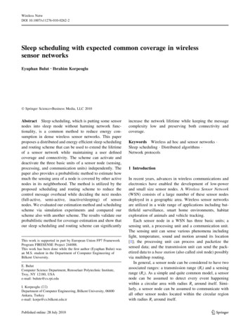
Wireless NetwAðTKMLÞ ¼ pR2t AðTKNLÞ Zy¼h qffiffiffiffiffiffiffiffiffiffiffiffiffiffiffi AðTKNLÞ ¼ 2Rt y Rs y þ x dyp¼þAðTKNLÞpR2tp ¼ E½pðXÞ ¼pffiffiffiWhen Rs 2 Rt 2Rs :x¼RZ t RsðRs Rt Þ2 fX ðxÞdxx¼0x¼RZ s Rt2þðRt Rs Þ fX ðxÞdxx¼0x¼xZ borderþx¼RZ sx¼RZ sp2 ðxÞ fX ðxÞdxx¼Rt Rsp2 ðxÞ fX ðxÞdxx¼Rs Rtþp1 ðxÞ fX ðxÞdxx¼xborderp¼pðxÞ fX ðxÞdxx¼RZ sþx¼0p ¼ E½pðXÞ ¼p2 ðxÞ fX ðxÞdxx¼Rt RsThe bordervalue xborder, that separates these cases �2equal to Rs R2t . As a result, when Rt \ Rs, the expectedvalue of the probability (E[p(X)]) that a point inside thesensing area is covered by a neighbor is:x¼RZ sðRs Rt Þ2 fX ðxÞdxx¼0x¼xZ bordery¼0p2 ðxÞ ¼ 1 x¼RZ t Rsp1 ðxÞ fX ðxÞdx where,x¼xborderfX ðxÞ ¼ 2x R2sIn other words, p expresses the expected commoncoverage between a node and one of its neighbors. WhenRt [ Rs we can find p in a similar way. But there are twodifferent calculations inpffiffithisffi case. The border case, whichhappens when Rt ¼ Rps ffiffiffi2, is illustrated in Fig. 4.When Rs Rt Rs 2:LNow, let pn;d1 ;d2 denote the expected overlap of a nodei’s sensing area by n nodes, where these nodes havedistance from the node in the interval [d1, d2]. And, let pndenote the expected overlap by n 1-hop neighbors. Then,pn ¼ pn;0;Rt . When n 1, it is equal to p0;Rt or simply p.Assume there are n nodes in interval [0, Rt] afterdeployment (i.e. n 1-hop neighbors). Then1,pn ¼ pn;0;Rt ¼x¼RZ sð1 ð1 pðxÞÞn Þ fX ðxÞdxx¼0We did some simulation experiments to check thevalidity of our estimation method. In our simulationexperiments, we created random multiple neighbors to anode within its transmission range and calculated theoverlap of the node’s sensing area by its neighbors.Besides, for each multiple neighbor count, the simulation isrun 1000 times and the result is obtained as the average ofthem. The Fig. 5 show the comparison of simulation andanalytical results for three different Rt/Rs values. As it canbe seen from the figure, the analytical results completelyoverlap with the simulation results.RtRsORsP1KFig. 4 Border case when Rt [ Rs123In this analysis, we assumed that the links between the nodes aremostly reliable and there are no frequent link failures which mayaffect the data acquisition significantly. However, we can reflect thefailure-prone nature of sensor node connections to this formula bymultiplying n by k (the probability that a connection between twoconnections may fail). Moreover, we can also include non-uniformnode distribution in the network by updating the density functionfX(x).

Wireless Netwx¼RZ s1p0;Rt ¼Expected Overlap0.9x¼00.8x¼RZ sp0;2Rt ¼0.7x¼0Simulation Rt/Rs 0.5Formula Rt/Rs 0.5Simulation Rt/Rs 1Formula Rt/Rs 1Simulation Rt/Rs 1.5Formula Rt/Rs 1.50.60.50.4123456x¼0Number of one hop neighborsFig. 5 Expected overlap values from simulation and formula withdifferent Rt/Rs ratios3.2 Expected common sensing coverage with 2-hopneighborsA sensor node may have not only 1-hop communicationneighbors but also two- or more hop communicationneighbors which have overlapping sensing area with itself.Especially, when the Rt/Rs value gets smaller, multi-hopneighbors may create a significant overlap on the node’ssensing area. To see the effect of multi-hop neighbors weneed to calculate expected overlap as in 1-hop neighbor case.Here, we calculate the expected overlap with only 2-hopneighbors. Computing expected overlap for more than twohops is more complex and we leave it out of the scope of thispaper. Additionally, as we discuss, using only 1-hop and2-hop neighbors addresses a wide range of realistic scenarios.Consider the Fig. 6. First, we will find the expectedoverlap by another node which has a distance to the node ofinterest in the interval [Rt, 2Rt]. As it is stated before, wedenote this with pRt ;2Rt . We can calculate this expectedvalue similar to 1-hop case as follows:¼AþBpð2Rt Þ2x¼RZ spRt ;2Rt ¼7AfX ðxÞdxpR2tfX ðxÞdxBpð2Rt Þ2 pRt 2fX ðxÞdx4p0;2Rt p0;Rt3For example, when Rt ¼ Rs ; p0;Rt ¼ 0:58 and p0;2Rt ¼0:25, then pRt ;2Rt ¼ ð4ð0:25Þ 0:58Þ 3 ¼ 0:13.Furthermore, if there are n such nodes (located at adistance in the interval [Rt, 2Rt]), the expected overlap bythese nodes is:pn;Rt ;2Rt ¼x¼RZ sx¼0 B n1 1 fX ðxÞdx3pR2tIn the above, note that, we found the expected overlapby possible 2-hop neighbors, i.e. nodes that are located ata distance between Rt and 2Rt. But for a node to be anactual 2-hop neighbor, being located at a distancebetween Rt and 2Rt is not sufficient because it shouldalso be in the transmission range of a 1-hop neighbor ofthe node.In Fig. 7, the existence of an actual 2-hop neighborat point P is possible with the existence of at least one1-hop neighbor in the shaded region. Following the samecalculation approach used before, given that there are n11-hop neighbors of the node, we conclude that theaverage probability (an1 ;Rt ) that there will be an actual2-hop neighbor at any point in the range [Rt, 2Rt] is:DLRsAOPRt2RtBMKEFig. 6 Expected overlap by a node located at a point P which has adistance to the node in the interval [Rt, 2Rt]Fig. 7 The probability that there will be a 2-hop neighbor at point Pis proportional with the probability that shaded area contains a 1-hopneighbor123

Wireless Netwan1 ;Rt ¼x¼2RZ tx¼Rty¼b¼2 2xn1ð1 ð1 bÞ Þ ;3R2twherepffiffiffiffiffiffiffiffiffiffi22 x Z Rt 4 ��2 Rt 2 y 2 x :y¼0Let pn1 ;n2 denote the expected overlap by n1 1-hop andn2 2-hop neighbors. Then, to find the value of pn1 ;n2 , weagain use the same probabilistic approach and combine theexpected overlap of each hop. For instance, if there are n11-hop neighbors and n2 2-hop neighbors, the expectedoverlap by 1-hop and 2-hop neighbors (pn1 ;n2 ) together canbe calculated as:x¼RZ s x¼0 A n1Ban1 ;Rt n21 1 21 fX ðxÞdxpRt3pR2tConsequently, when a node knows the number of 1-hopand 2-hop neighbors, it can find the expected overlap of itssensing area by these nodes.To check the validity of our analysis for 2-hop case, wealso did simulations. When Rs Rt, we found the expectedoverlap for different n1 and n2 values by using both analysis and simulation. Figure 8 shows the expected overlapfor a node for all cases when 1 n1 3 and 0 n2 6: AsFig. 8 shows, the results obtained with analysis arematching with simulation results. For instance, if a nodehas one 1-hop neighbor and two 2-hop neighbors, then itcan expect that 60.9% of its sensing area is covered bythese neighbors. Here, note that, the overlap shows only asmall increase with increasing n2. Moreover, the effectof 2-hop neighbors on the overlap decreases when n1increases. These two observations are expected because2-hop neighbors are located around 1-hop neighbors so that10.9Expected Overlap0.80.70.60.5Simulation n1 10.4Formula n 110.3Simulation n 21Formula n 20.21Simulation n 3the most part of the overlap resulting from 2-hop neighborsare already covered by 1-hop neighbors.At the beginning of a network deployment, if we knowthe Rt and Rs values, we can calculate the expected overlapvalues for different 1- and 2-hop neighbor counts into atable (we call it Expected Overlap Table) where cell(i, j) of the table shows the expected overlap with i 1-hopand j 2-hop neighbors, and install this table in each sensornode. Then during network operation, sensor nodes can usethe table to estimate the common coverage with theirneighbors at any moment by just using their count.4 Our combined sleep scheduling and routing schemeIn this section we introduce our combined sleep schedulingand routing scheme that works in a distributed and localized manner. It preserves both coverage and connectivity.It utilizes our probabilistic coverage estimation method,presented in the previous section, to reduce messagingoverhead while collecting status information from neighboring nodes.We assume all sensor nodes in the network are identicaland have the same Rt and Rs. Besides, we assume that allnodes know their locations. This may be achieved via GPSmodules or by use of localization algorithms [20, 21]. Wealso assume that nodes use data aggregation while forwarding the data they receive from their descendants. Thisis, however, not crucial. The scheme will work with nodata aggregation as well.Our combined sleep scheduling and routing schemeconsists of four phases; global tier assignment, neighborhood table construction, mode selection, and operationphases. Global tier assignment phase and neighborhoodtable construction phase run only at network setup time;and the mode selection and operation phases run in eachround (see Fig. 9).Our scheme requires network to operate in rounds. Around is a fixed time interval, determining the frequency ofmode re-assignments to nodes. A round consists of twophases executed sequentially one after another: modeselection phase and operation phase. Those two phases areof fixed length as well. The operation phase should bemuch longer than the mode selection phase. During modeselection phase, the mode of each node (which can eitherbe ON-DUTY, or TR-ON-DUTY, or DEEP-SLEEP) isdecided. During the operation phase, each node stays at the10.1Formula n 310012345Number of two hop neighbors (n2 )Fig. 8 Expected overlap values from simulation and formula withdifferent n1 and n2 counts and when Rt/Rs 1123round round 16StartGlobal TierAssignmentNeighborhood TableConstructionModeSelectionOperationFig. 9 Running order of the phases during the network lifetimeEnd

Wireless Netwdecided mode and data gathering from the sensor nodes tothe sink happens. The round duration and the duration of itsinner phases are same for all nodes and we assume allnodes are aware of this.At each round, modes are re-assigned to nodes. At thebeginning of each round, each node starts with a new modeselection phase where it

Wireless Netw 123. There are also various sleep scheduling schemes fol-lowing distributed approach. GAF [11] divides a region into equal-sized grid cells and tries to leave only one node active in each cell. In PEAS [12, 13], a node decides to go into