Transcription
11. Correlation and linear regressionThe goal in this chapter is to introduce correlation and linear regression. These are the standardtools that statisticians rely on when analysing the relationship between continuous predictors andcontinuous outcomes.11.1CorrelationsIn this section we’ll talk about how to describe the relationships between variables in the data. To dothat, we want to talk mostly about the correlation between variables. But first, we need some data.11.1.1The dataTable 11.1: Descriptive statistics for the parenthood data.variableminmax mean median std. dev IQRDan’s grumpiness419163.716210.0514Dan’s hours slept4.84 9.006.977.031.021.45Dan’s son’s hours slept 3.25 12.07 8.057.952.073.21.Let’s turn to a topic close to every parent’s heart: sleep. The data set we’ll use is fictitious,but based on real events. Suppose I’m curious to find out how much my infant son’s sleeping habitsaffect my mood. Let’s say that I can rate my grumpiness very precisely, on a scale from 0 (notat all grumpy) to 100 (grumpy as a very, very grumpy old man or woman). And lets also assumethat I’ve been measuring my grumpiness, my sleeping patterns and my son’s sleeping patterns for- 251 -
quite some time now. Let’s say, for 100 days. And, being a nerd, I’ve saved the data as a filecalled parenthood.csv. If we load the data into JASP we can see that the file contains four variablesdan.sleep, baby.sleep, dan.grump and day. Note that when you first load this data set JASP maynot have guessed the data type for each variable correctly, in which case you should fix it: dan.sleep,baby.sleep, dan.grump and day can be specified as continuous variables, and ID is a nominal(integer)variable.50607080My 51005Frequency2020Next, I’ll take a look at some basic descriptive statistics and, to give a graphical depiction of whateach of the three interesting variables looks like, Figure 11.1 plots histograms. One thing to note:just because JASP can calculate dozens of different statistics doesn’t mean you should report all ofthem. If I were writing this up for a report, I’d probably pick out those statistics that are of mostinterest to me (and to my readership), and then put them into a nice, simple table like the one inTable 11.1.1 Notice that when I put it into a table, I gave everything “human readable” names. Thisis always good practice. Notice also that I’m not getting enough sleep. This isn’t good practice, butother parents tell me that it’s pretty standard.5678My sleep (hours)(b)94681012The baby’s sleep (hours)(c)Figure 11.1: Histograms for the three interesting variables in the parenthood data set.11.1.2The strength and direction of a relationshipWe can draw scatterplots to give us a general sense of how closely related two variables are. Ideallythough, we might want to say a bit more about it than that. For instance, let’s compare the relationshipbetween dan.sleep and dan.grump (Figure 11.2, left) with that between baby.sleep and dan.grump(Figure 11.2, right). When looking at these two plots side by side, it’s clear that the relationship isqualitatively the same in both cases: more sleep equals less grump! However, it’s also pretty obviousthat the relationship between dan.sleep and dan.grump is stronger than the relationship between1Actually, even that table is more than I’d bother with. In practice most people pick one measure of central tendency,and one measure of variability only.- 252 -
9070405060My grumpiness80908070604050My grumpiness567894My sleep (hours)681012The baby’s sleep (hours)(a)(b)Figure 11.2: Scatterplots showing the relationship between dan.sleep and dan.grump (left) and therelationship between baby.sleep and dan.grump (right).baby.sleep and dan.grump. The plot on the left is “neater” than the one on the right. What it feelslike is that if you want to predict what my mood is, it’d help you a little bit to know how many hoursmy son slept, but it’d be more helpful to know how many hours I slept.In contrast, let’s consider the two scatterplots shown in Figure 11.3. If we compare the scatterplotof “ baby.sleep v dan.grump” (left) to the scatterplot of “ ‘baby.sleep v dan.sleep” (right), the overallstrength of the relationship is the same, but the direction is different. That is, if my son sleeps more,I get more sleep (positive relationship, right hand side), but if he sleeps more then I get less grumpy(negative relationship, left hand side).11.1.3The correlation coefficientWe can make these ideas a bit more explicit by introducing the idea of a correlation coefficient(or, more specifically, Pearson’s correlation coefficient), which is traditionally denoted as r . Thecorrelation coefficient between two variables X and Y (sometimes denoted rXY ), which we’ll definemore precisely in the next section, is a measure that varies from 1 to 1. When r “ 1 it meansthat we have a perfect negative relationship, and when r “ 1 it means we have a perfect positiverelationship. When r “ 0, there’s no relationship at all. If you look at Figure 11.4, you can see several- 253 -
99076My sleep (hours)880706040550My grumpiness46810124The baby’s sleep (hours)681012The baby’s sleep (hours)(a)(b)Figure 11.3: Scatterplots showing the relationship between baby.sleep and dan.grump (left), ascompared to the relationship between baby.sleep and dan.sleep (right).plots showing what different correlations look like.The formula for the Pearson’s correlation coefficient can be written in several different ways. I thinkthe simplest way to write down the formula is to break it into two steps. Firstly, let’s introducethe idea of a covariance. The covariance between two variables X and Y is a generalisation of thenotion of the variance amd is a mathematically simple way of describing the relationship betweentwo variables that isn’t terribly informative to humansCovpX, Y q “N 1 ÿ Xi X̄ Yi ȲN 1 i“1Because we’re multiplying (i.e., taking the “product” of) a quantity that depends on X by a quantitythat depends on Y and then averaginga , you can think of the formula for the covariance as an- 254 -
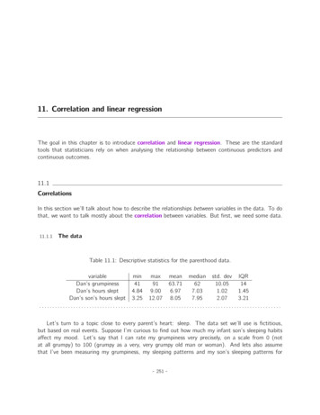
positive correlationsnegative correlations0.00.00.33 0.330.66 0.661.0 1.0Figure 11.4: Illustration of the effect of varying the strength and direction of a correlation. In the lefthand column, the correlations are 0, .33, .66 and 1. In the right hand column, the correlations are 0,-.33, -.66 and -1. . . . . . . . . . . . . . . . . . . . . . . . . . . . . . . . . . . . . . . . . . . -. .255. . . -. . . . . . . . . . . . . . . . . . . . . . . . . . . . . . . . . . . . . . . . . . . .
“average cross product” between X and Y .The covariance has the nice property that, if X and Y are entirely unrelated, then the covarianceis exactly zero. If the relationship between them is positive (in the sense shown in Figure 11.4) thenthe covariance is also positive, and if the relationship is negative then the covariance is also negative.In other words, the covariance captures the basic qualitative idea of correlation. Unfortunately, theraw magnitude of the covariance isn’t easy to interpret as it depends on the units in which X and Yare expressed and, worse yet, the actual units that the covariance itself is expressed in are really weird.For instance, if X refers to the dan.sleep variable (units: hours) and Y refers to the dan.grumpvariable (units: grumps), then the units for their covariance are “hours ˆ grumps”. And I have nofreaking idea what that would even mean.The Pearson correlation coefficient r fixes this interpretation problem by standardising the covariance, in pretty much the exact same way that the z-score standardises a raw score, by dividingby the standard deviation. However, because we have two variables that contribute to the covariance, the standardisation only works if we divide by both standard deviations.b In other words, thecorrelation between X and Y can be written as follows:rXY “abCovpX, Y qˆX ˆYJust like we saw with the variance and the standard deviation, in practice we divide by N 1 rather than N.This is an oversimplification, but it’ll do for our purposes.By standardising the covariance, not only do we keep all of the nice properties of the covariancediscussed earlier, but the actual values of r are on a meaningful scale: r “ 1 implies a perfect positiverelationship and r “ 1 implies a perfect negative relationship. I’ll expand a little more on this pointlater, in Section 11.1.5. But before I do, let’s look at how to calculate correlations in JASP.11.1.4Calculating correlations in JASPCalculating correlations in JASP can be done by clicking on the ‘Regression’ - ‘Correlation Matrix’button. Transfer all four continuous variables across into the box on the right to get the output inFigure 11.5. Notice that each correlation (denoted ‘Pearson’s r ’) is paired with a p-value. Clearly,something is being tested here, but ignore it for now. We’ll talk more about that soon!11.1.5Interpreting a correlationNaturally, in real life you don’t see many correlations of 1. So how should you interpret a correlationof, say, r “ .4? The honest answer is that it really depends on what you want to use the data for,and on how strong the correlations in your field tend to be. A friend of mine in engineering onceargued that any correlation less than .95 is completely useless (I think he was exaggerating, even for- 256 -
Figure 11.5: A JASP screenshot showing correlations between variables in the parenthood.csv file.engineering). On the other hand, there are real cases, even in psychology, where you should reallyexpect correlations that strong. For instance, one of the benchmark data sets used to test theoriesof how people judge similarities is so clean that any theory that can’t achieve a correlation of at least.9 really isn’t deemed to be successful. However, when looking for (say) elementary correlates ofintelligence (e.g., inspection time, response time), if you get a correlation above .3 you’re doing veryvery well. In short, the interpretation of a correlation depends a lot on the context. That said, therough guide in Table 11.2 is pretty typical.However, something that can never be stressed enough is that you should always look at thescatterplot before attaching any interpretation to the data. A correlation might not mean what youthink it means. The classic illustration of this is “Anscombe’s Quartet” (Anscombe 1973), a collectionof four data sets. Each data set has two variables, an X and a Y . For all four data sets the mean valuefor X is 9 and the mean for Y is 7.5. The standard deviations for all X variables are almost identical,as are those for the Y variables. And in each case the correlation between X and Y is r “ 0.816. Youcan verify this yourself, since I happen to have saved it in a file called anscombe.csv.You’d think that these four data sets would look pretty similar to one another. They do not. If wedraw scatterplots of X against Y for all four variables, as shown in Figure 11.6, we see that all fourof these are spectacularly different to each other. The lesson here, which so very many people seem- 257 -
Table 11.2: A rough guide to interpreting correlations. Note that I say a rough guide. There aren’thard and fast rules for what counts as strong or weak relationships. It depends on the context.Correlation StrengthDirection-1.0 to -0.9 Very strong Negative-0.9 to -0.7 StrongNegative-0.7 to -0.4 ModerateNegative-0.4 to -0.2 WeakNegative-0.2 to 0NegligibleNegative0 to 0.2NegligiblePositive0.2 to 0.4WeakPositive0.4 to 0.7ModeratePositive0.7 to 0.9StrongPositive0.9 to 1.0Very strong Positive.to forget in real life, is “always graph your raw data” (Chapter 5).11.1.6Spearman’s rank correlationsThe Pearson correlation coefficient is useful for a lot of things, but it does have shortcomings.One issue in particular stands out: what it actually measures is the strength of the linear relationshipbetween two variables. In other words, what it gives you is a measure of the extent to which thedata all tend to fall on a single, perfectly straight line. Often, this is a pretty good approximation towhat we mean when we say “relationship”, and so the Pearson correlation is a good thing to calculate.Sometimes though, it isn’t.One very common situation where the Pearson correlation isn’t quite the right thing to use ariseswhen an increase in one variable X really is reflected in an increase in another variable Y , but thenature of the relationship isn’t necessarily linear. An example of this might be the relationship betweeneffort and reward when studying for an exam. If you put zero effort (X) into learning a subject thenyou should expect a grade of 0% (Y ). However, a little bit of effort will cause a massive improvement.Just turning up to lectures means that you learn a fair bit, and if you just turn up to classes andscribble a few things down your grade might rise to 35%, all without a lot of effort. However, youjust don’t get the same effect at the other end of the scale. As everyone knows, it takes a lot moreeffort to get a grade of 90% than it takes to get a grade of 55%. What this means is that, if I’vegot data looking at study effort and grades, there’s a pretty good chance that Pearson correlationswill be misleading.To illustrate, consider the data plotted in Figure 11.7, showing the relationship between hoursworked and grade received for 10 students taking some class. The curious thing about this (highlyfictitious) data set is that increasing your effort always increases your grade. It might be by a lot- 258 -
9Y26789 4681012148X31012141618X4Figure 11.6: Anscombe’s quartet. All four of these data sets have a Pearson correlation of r “ .816,but they are qualitatively different from one another.or it might be by a little, but increasing effort will never decrease your grade. If we run a standardPearson correlation, it shows a strong relationship between hours worked and grade received, with acorrelation coefficient of 0.91. However, this doesn’t actually capture the observation that increasinghours worked always increases the grade. There’s a sense here in which we want to be able to saythat the correlation is perfect but for a somewhat different notion of what a “relationship” is. Whatwe’re looking for is something that captures the fact that there is a perfect ordinal relationship here.- 259 -
100806040020Grade Received020406080Hours WorkedFigure 11.7: The relationship between hours worked and grade received for a toy data set consisting ofonly 10 students (each circle corresponds to one student). The dashed line through the middle showsthe linear relationship between the two variables. This produces a strong Pearson correlation of r “ .91.However, the interesting thing to note here is that there’s actually a perfect monotonic relationshipbetween the two variables. In this toy example, increasing the hours worked always increases the gradereceived, as illustrated by the solid line. This is reflected in a Spearman correlation of “ 1. Withsuch a small data set, however, it’s an open question as to which version better describes the actualrelationship involved.That is, if student 1 works more hours than student 2, then we can guarantee that student 1 will getthe better grade. That’s not what a correlation of r “ .91 says at all.How should we address this? Actually, it’s really easy. If we’re looking for ordinal relationships allwe have to do is treat the data as if it were ordinal scale! So, instead of measuring effort in termsof “hours worked”, lets rank all 10 of our students in order of hours worked. That is, student 1 didthe least work out of anyone (2 hours) so they get the lowest rank (rank 1). Student 4 was thenext laziest, putting in only 6 hours of work over the whole semester, so they get the next lowest rank(rank 2). Notice that I’m using “rank 1” to mean “low rank”. Sometimes in everyday languagewe talk about “rank 1” to mean “top rank” rather than “bottom rank”. So be careful, you can rank“from smallest value to largest value” (i.e., small equals rank 1) or you can rank “from largest valueto smallest value” (i.e., large equals rank 1). In this case, I’m ranking from smallest to largest, but asit’s really easy to forget which way you set things up you have to put a bit of effort into remembering!- 260 -
Okay, so let’s have a look at our students when we rank them from worst to best in terms of effortand reward:rank (hours worked) rank (grade received)student 111student 21010student 366student 422student 533student 655student 744student 888student 977student 1099Hmm. These are identical. The student who put in the most effort got the best grade, the studentwith the least effort got the worst grade, etc. As the table above shows, these two rankings areidentical, so if we now correlate them we get a perfect relationship, with a correlation of 1.0.What we’ve just re-invented is Spearman’s rank order correlation, usually denoted to distinguishit from the Pearson correlation r . We can calculate Spearman’s using JASP simply by clicking the‘Spearman’ check box in the ‘Correlation Matrix’ screen.11.2ScatterplotsScatterplots are a simple but effective tool for visualising the relationship between two variables, likewe saw with the figures in the section on correlation (Section 11.1). It’s this latter application thatwe usually have in mind when we use the term “scatterplot”. In this kind of plot each observationcorresponds to one dot. The horizontal location of the dot plots the value of the observation on onevariable, and the vertical location displays its value on the other variable. In many situations you don’treally have a clear opinions about what the causal relationship is (e.g., does A cause B, or does Bcause A, or does some other variable C control both A and B). If that’s the case, it doesn’t reallymatter which variable you plot on the x-axis and which one you plot on the y-axis. However, in manysituations you do have a pretty strong idea which variable you think is most likely to be causal, orat least you have some suspicions in that direction. If so, then it’s conventional to plot the causevariable on the x-axis, and the effect variable on the y-axis. With that in mind, let’s look at how todraw scatterplots in JASP, using the same parenthood data set (i.e. parenthood.csv) that I usedwhen introducing correlations.Suppose my goal is to draw a scatterplot displaying the relationship between the amount of sleepthat I get (dan.sleep) and how grumpy I am the next day (dan.grump). The way in which we canuse JASP to get this plot is to use the ‘Plots’ option under the ‘Regression’ - ‘Correlation Matrix’- 261 -
Figure 11.8: Scatterplot via the ‘Correlation Matrix’ method in JASP.button, giving us the output shown in Figure 11.8. Note that JASP draws a line through the points,we’ll come onto this a bit later in Section (11.3). Plotting a scatterplot in this way also allow you tospecify ‘Densities for variables’, which adds a histogram and density curve showing how the data ineach variable is distributed. You can also specify the ‘Statistics’ option, which provides an estimateof the correlation along with a 95% confidence interval.11.3What is a linear regression model?Stripped to its bare essentials, linear regression models are basically a slightly fancier version of thePearson correlation (Section 11.1), though as we’ll see regression models are much more powerfultools.Since the basic ideas in regression are closely tied to correlation, we’ll return to the- 262 -
parenthood.csv file that we were using to illustrate how correlations work. Recall that, in this dataset we were trying to find out why Dan is so very grumpy all the time and our working hypothesis wasthat I’m not getting enough sleep. We drew some scatterplots to help us examine the relationshipbetween the amount of sleep I get and my grumpiness the following day, as in Figure 11.8, and aswe saw previously this corresponds to a correlation of r “ .90, but what we find ourselves secretlyimagining is something that looks closer to Figure 11.9a. That is, we mentally draw a straight linethrough the middle of the data. In statistics, this line that we’re drawing is called a regression line.Notice that, since we’re not idiots, the regression line goes through the middle of the data. We don’tfind ourselves imagining anything like the rather silly plot shown in Figure 11.9b.807060My grumpiness (0 100)40508070605040My grumpiness (0 100)90Not The Best Fitting Regression Line!90The Best Fitting Regression Line567895My sleep (hours)6789My sleep (hours)(a)(b)Figure 11.9: Panel a shows the sleep-grumpiness scatterplot from Figure 11.8 with the best fittingregression line drawn over the top. Not surprisingly, the line goes through the middle of the data. Incontrast, panel b shows the same data, but with a very poor choice of regression line drawn over thetop.This is not highly surprising. The line that I’ve drawn in Figure 11.9b doesn’t “fit” the data verywell, so it doesn’t make a lot of sense to propose it as a way of summarising the data, right? This isa very simple observation to make, but it turns out to be very powerful when we start trying to wrapjust a little bit of maths around it. To do so, let’s start with a refresher of some high school maths.The formula for a straight line is usually written like thisy “ a bxOr, at least, that’s what it was when I went to high school all those years ago. The two variables- 263 -
are x and y , and we have two coefficients, a and b.2 The coefficient a represents the y -interceptof the line, and coefficient b represents the slope of the line. Digging further back into our decayingmemories of high school (sorry, for some of us high school was a long time ago), we remember thatthe intercept is interpreted as “the value of y that you get when x “ 0”. Similarly, a slope of b meansthat if you increase the x-value by 1 unit, then the y -value goes up by b units, and a negative slopemeans that the y -value would go down rather than up. Ah yes, it’s all coming back to me now. Nowthat we’ve remembered that it should come as no surprise to discover that we use the exact sameformula for a regression line. If Y is the outcome variable (the DV) and X is the predictor variable(the IV), then the formula that describes our regression is written like thisŶi “ b0 b1 XiHmm. Looks like the same formula, but there’s some extra frilly bits in this version. Let’s make surewe understand them. Firstly, notice that I’ve written Xi and Yi rather than just plain old X and Y .This is because we want to remember that we’re dealing with actual data. In this equation, Xi is thevalue of predictor variable for the i th observation (i.e., the number of hours of sleep that I got on dayi of my little study), and Yi is the corresponding value of the outcome variable (i.e., my grumpinesson that day). And although I haven’t said so explicitly in the equation, what we’re assuming is thatthis formula works for all observations in the data set (i.e., for all i ). Secondly, notice that I wroteŶi and not Yi . This is because we want to make the distinction between the actual data Yi , and theestimate Ŷi (i.e., the prediction that our regression line is making). Thirdly, I changed the letters usedto describe the coefficients from a and b to b0 and b1 . That’s just the way that statisticians like torefer to the coefficients in a regression model. I’ve no idea why they chose b, but that’s what theydid. In any case b0 always refers to the intercept term, and b1 refers to the slope.Excellent, excellent. Next, I can’t help but notice that, regardless of whether we’re talking aboutthe good regression line or the bad one, the data don’t fall perfectly on the line. Or, to say it anotherway, the data Yi are not identical to the predictions of the regression model Ŷi . Since statisticianslove to attach letters, names and numbers to everything, let’s refer to the difference between themodel prediction and that actual data point as a residual, and we’ll refer to it as "i .3 Written usingmathematics, the residuals are defined as"i “ Yi Ŷiwhich in turn means that we can write down the complete linear regression model asYi “ b0 b1 Xi "i- 264 -
Regression Line Close to the Data90807060My grumpiness (0 100)40508070605040My grumpiness (0 100)90Regression Line Distant from the Data567895My sleep (hours)6789My sleep (hours)(a)(b)Figure 11.10: A depiction of the residuals associated with the best fitting regression line (panel a),and the residuals associated with a poor regression line (panel b). The residuals are much smaller forthe good regression line. Again, this is no surprise given that the good line is the one that goes rightthrough the middle of the data.11.4Estimating a linear regression modelOkay, now let’s redraw our pictures but this time I’ll add some lines to show the size of the residualfor all observations. When the regression line is good, our residuals (the lengths of the solid blacklines) all look pretty small, as shown in Figure 11.10a, but when the regression line is a bad one theresiduals are a lot larger, as you can see from looking at Figure 11.10b. Hmm. Maybe what we “want”in a regression model is small residuals. Yes, that does seem to make sense. In fact, I think I’ll goso far as to say that the “best fitting” regression line is the one that has the smallest residuals. Or,better yet, since statisticians seem to like to take squares of everything why not say that:The estimated regression coefficients, b̂0 and b̂1 , are those that minimisethe sum of the squared residuals, which we could either write as i pYi Ŷi q2 or as i "i 2 .Yes, yes that sounds even better. And since I’ve indented it like that, it probably means that this is the23Also sometimes written as y “ mx b where m is the slope coefficient and b is the intercept (constant) coefficient.The " symbol is the Greek letter epsilon. It’s traditional to use "i or ei to denote a residual.- 265 -
right answer. And since this is the right answer, it’s probably worth making a note of the fact that ourregression coefficients are estimates (we’re trying to guess the parameters that describe a population!),which is why I’ve added the little hats, so that we get b̂0 and b̂1 rather than b0 and b1 . Finally, Ishould also note that, since there’s actually more than one way to estimate a regression model, themore technical name for this estimation process is ordinary least squares (OLS) regression.At this point, we now have a concrete definition for what counts as our “best” choice of regressioncoefficients, b̂0 and b̂1 . The natural question to ask next is, if our optimal regression coefficients arethose that minimise the sum squared residuals, how do we find these wonderful numbers? The actualanswer to this question is complicated and doesn’t help you understand the logic of regression.4 Thistime I’m going to let you off the hook. Instead of showing you the long and tedious way first andthen “revealing” the wonderful shortcut that JASP provides, let’s cut straight to the chase and justuse JASP to do all the heavy lifting.11.4.1Linear regression in JASPTo run my linear regression, open up the ‘Regression’ - ‘Linear Regression’ analysis in JASP, usingthe parenthood.csv data file. Then specify dan.grump as the ‘Dependent Variable’ and dan.sleep asthe variable entered in the ‘Covariates’ box. This gives the results shown in Figure 11.11, showing anintercept b̂0 “ 125.956 and the slope b̂1 “ 8.937. In other words, the best-fitting regression linethat I plotted in Figure 11.9 has this formula:Ŷi “ 125.956 p 8.937 Xi q11.4.2Interpreting the estimated modelThe most important thing to be able to understand is how to interpret these coefficients. Let’s startwith b̂1 , the slope. If we remember the definition of the slope, a regression coefficient of b̂1 “ 8.94means that if I increase Xi by 1, then I’m decreasing Yi by 8.94. That is, each additional hour of sleepthat I gain will improve my mood, reducing my grumpiness by 8.94 grumpiness points. What aboutthe intercept? Well, since b̂0 corresponds to “the expected value of Yi when Xi equals 0”, it’s prettystraightforward. It implies that if I get zero hours of sleep (Xi “ 0) then my grumpiness will go off4Or at least, I’m assuming that it doesn’t help most people. But on the off chance that someone reading this is aproper kung fu master of linear algebra (and to be fair, I always have a few of these people in my intro stats class), itwill help you to know that the solution to the estimation problem turns out to be b̂ “ pX1 Xq 1 X1 y, where b̂ is a vectorcontaining the estimated regression coefficients, X is the “design matrix” that contains the predictor variables (plus anadditional column containing all ones; strictly X is a matrix of the regressors, but I haven’t discussed the distinction yet),and y is a v
The baby’s sleep (hours) My grumpiness 4 6 8 10 12 567 89 The baby’s sleep (hours) My sleep (hours) (a) (b) Figure 11.3: Scatterplots showing the relationship between baby.sleep and dan.grump (left), as compared to the relationship b