Transcription
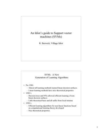
An Idiot’s guide to Support vectormachines (SVMs)R. Berwick, Village IdiotSVMs: A NewGeneration of Learning Algorithms Pre 1980:– Almost all learning methods learned linear decision surfaces.– Linear learning methods have nice theoretical properties 1980’s– Decision trees and NNs allowed efficient learning of nonlinear decision surfaces– Little theoretical basis and all suffer from local minima 1990’s– Efficient learning algorithms for non-linear functions basedon computational learning theory developed– Nice theoretical properties.1
Key Ideas Two independent developments within last decade– New efficient separability of non-linear regions that use“kernel functions” : generalization of ‘similarity’ tonew kinds of similarity measures based on dot products– Use of quadratic optimization problem to avoid ‘localminimum’ issues with neural nets– The resulting learning algorithm is an optimizationalgorithm rather than a greedy searchOrganization Basic idea of support vector machines: just like 1layer or multi-layer neural nets– Optimal hyperplane for linearly separablepatterns– Extend to patterns that are not linearlyseparable by transformations of original data tomap into new space – the Kernel function SVM algorithm for pattern recognition2
Support Vectors Support vectors are the data points that lie closestto the decision surface (or hyperplane) They are the data points most difficult to classify They have direct bearing on the optimum locationof the decision surface We can show that the optimal hyperplane stemsfrom the function class with the lowest“capacity” # of independent features/parameterswe can twiddle [note this is ‘extra’ material notcovered in the lectures you don’t have to knowthis]Recall from 1-layer nets : Which SeparatingHyperplane? In general, lots of possiblesolutions for a,b,c (aninfinite number!) Support Vector Machine(SVM) finds an optimalsolution3
Support Vector Machine (SVM) SVMs maximize the margin(Winston terminology: the ‘street’)around the separating hyperplane. The decision function is fullyspecified by a (usually very small)subset of training samples, thesupport vectors. This becomes a Quadraticprogramming problem that is easyto solve by standard methodsSupport vectorsMaximizemarginSeparation by Hyperplanes Assume linear separability for now (we will relax thislater) in 2 dimensions, can separate by a line– in higher dimensions, need hyperplanes4
General input/output for SVMs just like forneural nets, but for one important addition Input: set of (input, output) training pair samples; call theinput sample features x1, x2 xn, and the output result y.Typically, there can be lots of input features xi.Output: set of weights w (or wi), one for each feature,whose linear combination predicts the value of y. (So far,just like neural nets )Important difference: we use the optimization of maximizingthe margin (‘street width’) to reduce the number of weightsthat are nonzero to just a few that correspond to theimportant features that ‘matter’ in deciding the separatingline(hyperplane) these nonzero weights correspond to thesupport vectors (because they ‘support’ the separatinghyperplane)2-D CaseFind a,b,c, such thatax by c for red pointsax by (or ) c for greenpoints.5
Which Hyperplane to pick? Lots of possible solutions for a,b,c. Some methods find a separatinghyperplane, but not the optimal one (e.g.,neural net) But: Which points should influenceoptimality?– All points? Linear regression Neural nets– Or only “difficult points” close todecision boundary Support vector machinesSupport Vectors again for linearly separable case Support vectors are the elements of the training set thatwould change the position of the dividing hyperplane ifremoved. Support vectors are the critical elements of the training set The problem of finding the optimal hyper plane is anoptimization problem and can be solved by optimizationtechniques (we use Lagrange multipliers to get thisproblem into a form that can be solved analytically).6
Support Vectors: Input vectors that just touch the boundary of themargin (street) – circled below, there are 3 of them (or, rather, the‘tips’ of the vectorsw0 T x b 0 1orw0Tx b0 –1dXXXXXXHere, we have shown the actual support vectors, v1, v2, v3, instead ofjust the 3 circled points at the tail ends of the support vectors. ddenotes 1/2 of the street ‘width’dXXv1v2Xv3XXX7
DefinitionsDefine the hyperplanes H such that:w xi b 1 when yi 1w xi b -1 when yi –1H1 and H2 are the planes:H1: w xi b 1H2: w xi b –1H1H0H2d d-HThe points on the planes H1 andH2 are the tips of the SupportVectorsThe plane H0 is the median inbetween, where w xi b 0d the shortest distance to the closest positive pointd- the shortest distance to the closest negative pointThe margin (gutter) of a separating hyperplane is d d–.Moving a support vectormoves the decisionboundaryMoving the other vectorshas no effectThe optimization algorithm to generate the weights proceeds in such away that only the support vectors determine the weights and thus theboundary8
Defining the separating Hyperplane Form of equation defining the decision surface separatingthe classes is a hyperplane of the form:wTx b 0– w is a weight vector– x is input vector– b is bias Allows us to writewTx b 0 for di 1wTx b 0 for di –1Some final definitions Margin of Separation (d): the separation between thehyperplane and the closest data point for a given weightvector w and bias b. Optimal Hyperplane (maximal margin): the particularhyperplane for which the margin of separation d ismaximized.9
Maximizing the margin (aka street width)We want a classifier (linear separator)with as big a margin as possible.H0Recall the distance from a point(x0,y0) to a line:Ax By c 0 is: Ax0 By0 c /sqrt(A2 B2), so,The distance between H0 and H1 is then: w x b / w 1/ w , soH1H2d d-The total distance between H1 and H2 is thus: 2/ w In order to maximize the margin, we thus need to minimize w . With thecondition that there are no datapoints between H1 and H2:xi w b 1 when yi 1xi w b –1 when yi –1Can be combined into: yi(xi w) 1We now must solve a quadraticprogramming problem Problem is: minimize w , s.t. discrimination boundary isobeyed, i.e., min f(x) s.t. g(x) 0, which we can rewrite as:min f: ½ w 2 (Note this is a quadratic function)s.t. g: yi(w xi)–b 1 or [yi(w xi)–b] – 1 0This is a constrained optimization problemIt can be solved by the Lagrangian multipler methodBecause it is quadratic, the surface is a paraboloid, with just asingle global minimum (thus avoiding a problem we hadwith neural nets!)10
flattenExample: paraboloid 2 x2 2y2 s.t. x y 1Intuition: find intersection of two functions f, g ata tangent point (intersection both constraintssatisfied; tangent derivative is 0); this will be amin (or max) for f s.t. the contraint g is satisfiedFlattened paraboloid f: 2x2 2y2 0 with superimposedconstraint g: x y 1Minimize when the constraint line g (shown in green)is tangent to the inner ellipse contour linez of f (shown in red) –note direction of gradient arrows.11
flattened paraboloid f: 2 x2 2y2 0 with superimposed constraintg: x y 1; at tangent solution p, gradient vectors of f,g areparallel (no possible move to increment f that also keeps you inregion g)Minimize when the constraint line g is tangent to the inner ellipsecontour line of fTwo constraints1. Parallel normal constraint ( gradient constrainton f, g s.t. solution is a max, or a min)2. g(x) 0 (solution is on the constraint line as well)We now recast these by combining f, g as the newLagrangian function by introducing new ‘slackvariables’ denoted a or (more usually, denoted αin the literature)12
Redescribing these conditions Want to look for solution point p where"f ( p ) "! g ( p )g ( x) 0 Or, combining these two as the Langrangian L &requiring derivative of L be zero:L(x, a) f (x) ! ag(x)"(x, a) 0At a solution p The the constraint line g and the contour lines of f mustbe tangent If they are tangent, their gradient vectors(perpendiculars) are parallel Gradient of g must be 0 – i.e., steepest ascent & soperpendicular to f Gradient of f must also be in the same direction as g13
How Langrangian solves constrainedoptimizationL(x, a) f (x) ! ag(x) where"(x, a) 0Partial derivatives wrt x recover the parallel normalconstraintPartial derivatives wrt λ recover the g(x,y) 0In general,L(x, a) f (x) ! i ai g i (x)In generalGradient min of fconstraint condition gL(x, a) f (x) ! i ai g i (x) a function of n m variablesn for the x 's, m for the a. Differentiating gives n m equations, eachset to 0. The n eqns differentiated wrt each xi give the gradient conditions;the m eqns differentiated wrt each ai recover the constraints g iIn our case, f(x): ½ w 2 ; g(x): yi(w xi b)–1 0 so Lagrangian is:min L ½ w 2 – Σai[yi(w xi b)–1] wrt w, bWe expand the last to get the following L form:min L ½ w 2 – Σaiyi(w xi b) Σai wrt w, b14
Lagrangian Formulation So in the SVM problem the Lagrangian ismin LP 12l()lw ! " ai yi x i # w b " ai2i 1i 1s.t. i, ai % 0 where l is the # of training points From the property that the derivatives at min 0l!LPwe get: w" ayx 0#!wi 1l!LP " ai yi 0 so!bi 1lw ! ai yi x i ,i 1i iil!a yii 0i 1What’s with this Lp business? This indicates that this is the primal form of theoptimization problem We will actually solve the optimization problemby now solving for the dual of this originalproblem What is this dual formulation?15
The Lagrangian Dual Problem: instead of minimizing over w, b,subject to constraints involving a’s, we can maximize over a (thedual variable) subject to the relations obtained previously for wand bOur solution must satisfy these two relations:llw ! ai yi x i ,!a yii 1i 0i 1By substituting for w and b back in the original eqn we can get rid of thedependence on w and b.Note first that we already now have our answer for what the weights wmust be: they are a linear combination of the training inputs and thetraining outputs, xi and yi and the values of a. We will now solve for thea’s by differentiating the dual problem wrt a, and setting it to zero. Mostof the a’s will turn out to have the value zero. The non-zero a’s willcorrespond to the support vectorsPrimal problem:min LP l()lw ! " ai yi x i # w b " ai212i 1i 1s.t. i a i % 0lw ! ai yi x i ,i 1Dual problem:lmax LD (ai ) ! ai "i 1ls.t.!a yiil!a yii 0i 1(1 l!a a y y x #x2 i 1 i j i j i j) 0 & ai 0i 1(note that we have removed the dependence on w and b)16
The Dual problem Kuhn-Tucker theorem: the solution we find here willbe the same as the solution to the original problem Q: But why are we doing this? (why not justsolve the original problem?) Ans: Because this will let us solve the problem bycomputing the just the inner products of xi, xj (whichwill be very important later on when we want tosolve non-linearly separable classification problems)The Dual ProblemDual problem:lmax LD (ai ) ! ai "i 1ls.t.!a yii(1 l!a a y y x #x2 i 1 i j i j i j) 0 & ai 0i 1Notice that all we have are the dot products of xi,xjIf we take the derivative wrt a and set it equal to zero,we get the following solution, so we can solve for ai:l!a yi 1i i 00 " ai " C17
Now knowing the ai we can find theweights w for the maximal marginseparating hyperplane:lw ! ai yi x ii 1And now, after training and finding the w by this method,given an unknown point u measured on features xi wecan classify it by looking at the sign of:lf (x) wiu b (! ai yi x i iu) bi 1Remember: most of the weights wi, i.e., the a’s, will be zeroOnly the support vectors (on the gutters or margin) will have nonzeroweights or a’s – this reduces the dimensionality of the solutionInner products, similarity, and SVMsWhy should inner product kernels be involved in patternrecognition using SVMs, or at all?– Intuition is that inner products provide some measure of‘similarity’– Inner product in 2D between 2 vectors of unit length returns thecosine of the angle between them how ‘far apart’ they aree.g. x [1, 0]T , y [0, 1]Ti.e. if they are parallel their inner product is 1 (completely similar)xT y x y 1If they are perpendicular (completely unlike) their inner product is0 (so should not contribute to the correct classifier)xT y x y 018
Insight into inner productsConsider that we are trying to maximize the form:lLD (ai ) ! ai "i 1ls.t.!a yii(1 l!a a y y x #x2 i 1 i j i j i j) 0 & ai 0i 1The claim is that this function will be maximized if we give nonzero values to a’s thatcorrespond to the support vectors, ie, those that ‘matter’ in fixing the maximum widthmargin (‘street’). Well, consider what this looks like. Note first from the constraintcondition that all the a’s are positive. Now let’s think about a few cases.Case 1. If two features xi , xj are completely dissimilar, their dot product is 0, and they don’tcontribute to L.Case 2. If two features xi,xj are completely alike, their dot product is 0. There are 2 subcases.Subcase 1: both xi,and xj predict the same output value yi (either 1 or –1). Then yix yj is always 1, and the value of aiajyiyjxixj will be positive. But this would decrease thevalue of L (since it would subtract from the first term sum). So, the algorithm downgradessimilar feature vectors that make the same prediction.Subcase 2: xi,and xj make opposite predictions about the output value yi (ie, one is 1, the other –1), but are otherwise very closely similar: then the product aiajyiyjxix isnegative and we are subtracting it, so this adds to the sum, maximizing it. This is preciselythe examples we are looking for: the critical ones that tell the two classses apart.Insight into inner products, graphically: 2 veryvery similar xi, xj vectors that predict difftclasses tend to maximize the margin widthxixj19
2 vectors that are similar but predict thesame class are redundantxixj2 dissimilar (orthogonal) vectors don’tcount at allxjxi20
But are we done?Not Linearly Separable!Find a line that penalizespoints on “the wrong side”21
Transformation to separateϕo xxoxoxoxoxoϕ (x)ϕ (o)ϕ (x)ϕ (x)ϕ (o)ϕ (o)ϕ (x)ϕ (x)ϕ (o) ϕ (x)ϕ (o)ϕ (x)ϕ(o)ϕ (o)xXFNon–Linear SVMs The idea is to gain linearly separation by mapping the data toa higher dimensional space– The following set can’t be separated by a linear function,but can be separated by a quadratic one(x ! a )(x ! b ) x 2 ! (a b ) x abab{ }– So if we map x ! x 2 , xwe gain linear separation22
Problems with linear SVM -1 1What if the decision function is not linear? What transform would separate these?Ans: polar coordinates!Non-linear SVMThe Kernel trickImagine a function φ that maps the data into another space:Radialφ Radial ΗφΗ -1 1 -1 1Remember the function we want to optimize: Ld ai – ½ ai ajyiyj (xi xj) where (xi xj) is thedot product of the two feature vectors. If we now transform to φ, instead of computing thisdot product (xi xj) we will have to compute (φ (xi) φ (xj)). But how can we do this? This isexpensive and time consuming (suppose φ is a quartic polynomial or worse, we don’t know thefunction explicitly. Well, here is the neat thing:If there is a ”kernel function” K such that K(xi,xj) φ (xi) φ (xj), then we do not need to knowor compute φ at all!! That is, the kernel function defines inner products in the transformed space.Or, it defines similarity in the transformed space.23
Non-linear SVMsSo, the function we end up optimizing is:Ld ai – ½ aiaj yiyjK(xi xj),Kernel example: The polynomial kernelK(xi,xj) (xi xj 1)p, where p is a tunable parameterNote: Evaluating K only requires one addition and one exponentiationmore than the original dot productExamples for Non Linear SVMsK (x, y ) (x ! y 1)p{K (x, y ) exp "x"y22! 2}K (x, y ) tanh (! x # y " )1st is polynomial (includes x x as special case)2nd is radial basis function (gaussians)3rd is sigmoid (neural net activation function)24
We’ve already seen such nonlineartransforms What is it? tanh(β0xTxi β1) It’s the sigmoidtransform (for neuralnets) So, SVMs subsumeneural nets! (but w/otheir problems )Inner Product KernelsType of Support VectorMachineInner Product KernelK(x,xi ), I 1, 2, , NUsual inner productPolynomial learningmachine(xT xi 1)pPower p is specified apriori by the userRadial-basis function(RBF)exp(1/(2σ2) x-xi 2)The width σ2 isspecified a prioriTwo layer neural nettanh(β0 xTxi β1)Actually works only forsome values of β0 andβ125
Kernels generalize the notion of ‘innerproduct similarity’Note that one can define kernels over more than justvectors: strings, trees, structures, in fact, just aboutanythingA very powerful idea: used in comparing DNA, proteinstructure, sentence structures, etc.Examples for Non Linear SVMs 2 –Gaussian KernelLinearGaussian26
Nonlinear rbf kernelAdmiral’s delight w/ difft kernelfunctions27
Overfitting by SVMEvery point is a support vector too much freedom to bend to fit thetraining data – no generalization.In fact, SVMs have an ‘automatic’ way to avoid such issues, but wewon’t cover it here see the book by Vapnik, 1995. (We add apenalty function for mistakes made after training by over-fitting: recallthat if one over-fits, then one will tend to make errors on new data.This penalty fn can be put into the quadratic programming problemdirectly. You don’t need to know this for this course.)28
R. Berwick, Village Idiot SVMs: A New Generation of Learning Algorithms Pre 1980: –Almost all learning methods learned linear decision surfaces. –Linear learning methods have nice theoretical properties 1980’