Transcription
ANALOG FILTERSCHAPTER 8 ANALOG FILTERSSECTION 8.1: INTRODUCTIONSECTION 8.2: THE TRANSFER FUNCTIONTHE S-PLANEFO and QHIGH-PASS FILTERBAND-PASS FILTERBAND-REJECT (NOTCH) FILTERALL-PASS FILTERPHASE RESPONSETHE EFFECT OF NONLINEAR PHASESECTION 8.3: TIME DOMAIN RESPONSEIMPULSE RESPONSESTEP RESPONSESECTION 8.4: STANDARD RESPONSESBUTTERWORTHCHEBYSHEVBESSELLINEAR PHASE with EQUIRIPPLE ERRORTRANSITIONAL FILTERSCOMPARISON OF ALL-POLE RESPONSESELLIPTICALMAXIMALLY FLAT DELAY with CHEBYSHEV STOP BANDINVERSE CHEBYSHEVUSING THE PROTOTYPE RESPONSE CURVESRESPONSE CURVESBUTTERWORTH RESPONSE0.01 dB CHEBYSHEV RESPONSE0.1 dB CHEBYSHEV RESPONSE0.25 dB CHEBYSHEV RESPONSE0.5 dB CHEBYSHEV RESPONSE1 dB CHEBYSHEV RESPONSEBESSEL RESPONSELINEAR PHASE with EQUIRIPPLE ERROR of 0.05 RESPONSELINEAR PHASE with EQUIRIPPLE ERROR of 0.5 RESPONSEGAUSSIAN TO 12 dB RESPONSEGAUSSIAN TO 6 dB 318.328.338.348.358.368.278.388.398.408.41
BASIC LINEAR DESIGNSECTION 8.4: STANDARD RESPONSES (cont.)DESIGN TABLESBUTTERWORTH DESIGN TABLE0.01 dB CHEBYSHEV DESIGN TABLE0.1 dB CHEBYSHEV DESIGN TABLE0.25 dB CHEBYSHEV DESIGN TABLE0.5 dB CHEBYSHEV DESIGN TABLE1 dB CHEBYSHEV DESIGN TABLEBESSEL DESIGN TABLELINEAR PHASE with EQUIRIPPLE ERROR of 0.05 DESIGNTABLELINEAR PHASE with EQUIRIPPLE ERROR of 0.5 DESIGNTABLEGAUSSIAN TO 12 dB DESIGN TABLEGAUSSIAN TO 6 dB DESIGN TABLESECTION 8.5: FREQUENCY TRANSFORMATIONLOW-PASS TO HIGH-PASSLOW-PASS TO BAND-PASSLOW-PASS TO BAND-REJECT (NOTCH)LOW-PASS TO ALL-PASSSECTION 8.6: FILTER REALIZATIONSSINGLE POLE RCPASSIVE LC SECTIONINTEGRATORGENERAL IMPEDANCE CONVERTERACTIVE INDUCTORFREQUENCY DEPENDENT NEGATIVE RESISTOR (FDNR)SALLEN-KEYMULTIPLE FEEDBACKSTATE VARIABLEBIQUADRATIC (BIQUAD)DUAL AMPLIFIER BAND-PASS (DABP)TWIN T NOTCHBAINTER NOTCHBOCTOR NOTCH1 BAND-PASS NOTCHFIRST ORDER ALL-PASSSECOND ORDER 8.728.758.778.798.808.818.828.838.858.868.87
ANALOG FILTERSSECTION 8.6: FILTER REALIZATIONS (cont.)DESIGN PAGESSINGLE-POLESALLEN-KEY LOW-PASSSALLEN-KEY HIGH-PASSSALLEN-KEY BAND-PASSMULTIPLE FEEDBACK LOW-PASSMULTIPLE FEEDBACK HIGH-PASSMULTIPLE FEEDBACK BAND-PASSSTATE VARIABLEBIQUADDUAL AMPLIFIER BAND-PASSTWIN T NOTCHBAINTER NOTCHBOCTOR NOTCH (LOW-PASS)BOCTOR NOTCH (HIGH-PASS)FIRST ORDER ALL-PASSSECOND ORDER ALL-PASSSECTION 8.7: PRACTICAL PROBLEMS IN FILTERIMPLEMENTATIONPASSIVE COMPONENTSLIMITATIONS OF ACTIVE ELEMENTS (OP AMPS) IN FILTERSDISTORTION RESULTING FROM INPUT CAPACITANCEMODULATIONQ PEAKING AND Q ENHANSEMENTSECTION 8.8: DESIGN EXAMPLESANTIALIASING FILTERTRANSFORMATIONSCD RECONSTRUCTION FILTERDIGITALLY PROGRAMMABLE STATE VARIABLE FILTER60 HZ. NOTCH 148.1158.1178.1218.1218.1288.1348.1378.1418.143
BASIC LINEAR DESIGN
ANALOG FILTERSINTRODUCTIONCHAPTER 8: ANALOG FILTERSSECTION 8.1: INTRODUCTIONFilters are networks that process signals in a frequency-dependent manner. The basicconcept of a filter can be explained by examining the frequency dependent nature of theimpedance of capacitors and inductors. Consider a voltage divider where the shunt leg isa reactive impedance. As the frequency is changed, the value of the reactive impedancechanges, and the voltage divider ratio changes. This mechanism yields the frequencydependent change in the input/output transfer function that is defined as the frequencyresponse.Filters have many practical applications. A simple, single-pole, low-pass filter (theintegrator) is often used to stabilize amplifiers by rolling off the gain at higherfrequencies where excessive phase shift may cause oscillations.A simple, single-pole, high-pass filter can be used to block dc offset in high gainamplifiers or single supply circuits. Filters can be used to separate signals, passing thoseof interest, and attenuating the unwanted frequencies.An example of this is a radio receiver, where the signal you wish to process is passedthrough, typically with gain, while attenuating the rest of the signals. In data conversion,filters are also used to eliminate the effects of aliases in A/D systems. They are used inreconstruction of the signal at the output of a D/A as well, eliminating the higherfrequency components, such as the sampling frequency and its harmonics, thussmoothing the waveform.There are a large number of texts dedicated to filter theory. No attempt will be made togo heavily into much of the underlying math: Laplace transforms, complex conjugatepoles and the like, although they will be mentioned.While they are appropriate for describing the effects of filters and examining stability, inmost cases examination of the function in the frequency domain is more illuminating.An ideal filter will have an amplitude response that is unity (or at a fixed gain) for thefrequencies of interest (called the pass band) and zero everywhere else (called the stopband). The frequency at which the response changes from passband to stopband isreferred to as the cutoff frequency.Figure 8.1(A) shows an idealized low-pass filter. In this filter the low frequencies are inthe pass band and the higher frequencies are in the stop band.8.1
BASIC LINEAR DESIGNMAGNITUDEMAGNITUDEThe functional complement to the low-pass filter is the high-pass filter. Here, the lowfrequencies are in the stop-band, and the high frequencies are in the pass band.Figure 8.1(B) shows the idealized high-pass filter.fcfcFREQUENCYFREQUENCYMAGNITUDE(B) HighpassMAGNITUDE(A) Lowpassf1fh(C) BandpassFREQUENCYf1fhFREQUENCY(D) Notch (Bandreject)Figure 8.1: Idealized Filter ResponsesIf a high-pass filter and a low-pass filter are cascaded, a band pass filter is created. Theband pass filter passes a band of frequencies between a lower cutoff frequency, f l, and anupper cutoff frequency, f h. Frequencies below f l and above f h are in the stop band. Anidealized band pass filter is shown in Figure 8.1(C).A complement to the band pass filter is the band-reject, or notch filter. Here, the passbands include frequencies below f l and above f h. The band from f l to f h is in the stopband. Figure 8.1(D) shows a notch response.The idealized filters defined above, unfortunately, cannot be easily built. The transitionfrom pass band to stop band will not be instantaneous, but instead there will be atransition region. Stop band attenuation will not be infinite.The five parameters of a practical filter are defined in Figure 8.2, opposite.The cutoff frequency (Fc) is the frequency at which the filter response leaves the errorband (or the 3 dB point for a Butterworth response filter). The stop band frequency (Fs)is the frequency at which the minimum attenuation in the stopband is reached. The passband ripple (Amax) is the variation (error band) in the pass band response. The minimumpass band attenuation (Amin) defines the minimum signal attenuation within the stopband. The steepness of the filter is defined as the order (M) of the filter. M is also thenumber of poles in the transfer function. A pole is a root of the denominator of thetransfer function. Conversely, a zero is a root of the numerator of the transfer function.8.2
ANALOG FILTERSINTRODUCTIONEach pole gives a –6 dB/octave or –20 dB/decade response. Each zero gives a 6 dB/octave, or 20 dB/decade response.PASSBANDRIPPLEA MAX3dB POINTORCUTOFF FREQUENCYFcSTOPBANDATTENUATIONA MINSTOPBANDFREQUENCYFsPASS BANDSTOP BANDTRANSITIONBANDFigure 8.2: Key Filter ParametersNote that not all filters will have all these features. For instance, all-pole configurations(i.e. no zeros in the transfer function) will not have ripple in the stop band. Butterworthand Bessel filters are examples of all-pole filters with no ripple in the pass band.Typically, one or more of the above parameters will be variable. For instance, if you wereto design an antialiasing filter for an ADC, you will know the cutoff frequency (themaximum frequency that you want to pass), the stop band frequency, (which willgenerally be the Nyquist frequency ( ½ the sample rate)) and the minimum attenuationrequired (which will be set by the resolution or dynamic range of the system). You canthen go to a chart or computer program to determine the other parameters, such as filterorder, F0, and Q, which determines the peaking of the section, for the various sectionsand/or component values.It should also be pointed out that the filter will affect the phase of a signal, as well as theamplitude. For example, a single-pole section will have a 90 phase shift at the crossoverfrequency. A pole pair will have a 180 phase shift at the crossover frequency. The Q ofthe filter will determine the rate of change of the phase. This will be covered more indepth in the next section.8.3
BASIC LINEAR DESIGNNotes:8.4
ANALOG FILTERSTHE TRANSFER FUNCTIONSECTION 8.2: THE TRANSFER FUNCTIONThe S-PlaneFilters have a frequency dependent response because the impedance of a capacitor or aninductor changes with frequency. Therefore the complex impedances:ZL s LEq. 8-1andZC Eq. 8-21sCare used to describe the impedance of an inductor and a capacitor, respectively,s σ jωEq. 8-3where σ is the Neper frequency in nepers per second (NP/s) and ω is the angularfrequency in radians per sec (rad/s).By using standard circuit analysis techniques, the transfer equation of the filter can bedeveloped. These techniques include Ohm’s law, Kirchoff’s voltage and current laws,and superposition, remembering that the impedances are complex. The transfer equationis then:H(s) amsm am-1sm-1 a1s a0bnsn bn-1sn-1 b1s b0Eq. 8-4Therefore, H(s) is a rational function of s with real coefficients with the degree of m forthe numerator and n for the denominator. The degree of the denominator is the order ofthe filter. Solving for the roots of the equation determines the poles (denominator) andzeros (numerator) of the circuit. Each pole will provide a –6 dB/octave or –20 dB/decaderesponse. Each zero will provide a 6 dB/octave or 20 dB/decade response. These rootscan be real or complex. When they are complex, they occur in conjugate pairs. Theseroots are plotted on the s plane (complex plane) where the horizontal axis is σ (real axis)and the vertical axis is ω (imaginary axis). How these roots are distributed on the s planecan tell us many things about the circuit. In order to have stability, all poles must be inthe left side of the plane. If we have a zero at the origin, that is a zero in the numerator,the filter will have no response at dc (high-pass or band pass).Assume an RLC circuit, as in Figure 8.3. Using the voltage divider concept it can beshown that the voltage across the resistor is:H (s) Vo V inRCsLC s2 R C s 1Eq. 8-58.5
BASIC LINEAR DESIGN10mH10µF 10ΩVOUTFigure 8.3: RLC CircuitSubstituting the component values into the equation yields:H(s) 103 xsEq. 8-6s2 103s 107Factoring the equation and normalizing gives:H(s) 103 xs[ s - ( -0.5 j 3.122 ) x 103] x[ s - ( -0.5 - j 3.122 ) x 103]Im (krad / s)X 3.122Re (kNP / s)–0.5X–3.122Figure 8.4: Pole and Zero Plotted on the s-Plane8.6Eq 8-7
ANALOG FILTERSTHE TRANSFER FUNCTIONThis gives a zero at the origin and a pole pair at:s (-0.5 j3.122) x 103Eq. 8-8Next, plot these points on the s plane as shown in Figure 8.4:The above discussion has a definite mathematical flavor. In most cases we are moreinterested in the circuit’s performance in real applications. While working in the s planeis completely valid, I’m sure that most of us don’t think in terms of Nepers and imaginaryfrequencies.Fo and QSo if it is not convenient to work in the s plane, why go through the above discussion?The answer is that the groundwork has been set for two concepts that will be infinitelymore useful in practice: Fo and Q.Fo is the cutoff frequency of the filter. This is defined, in general, as the frequency wherethe response is down 3 dB from the pass band. It can sometimes be defined as thefrequency at which it will fall out of the pass band. For example, a 0.1 dB Chebyshevfilter can have its Fo at the frequency at which the response is down 0.1 dB.The shape of the attenuation curve (as well as the phase and delay curves, which definethe time domain response of the filter) will be the same if the ratio of the actual frequencyto the cutoff frequency is examined, rather than just the actual frequency itself.Normalizing the filter to 1 rad/s, a simple system for designing and comparing filters canbe developed. The filter is then scaled by the cutoff frequency to determine thecomponent values for the actual filter.Q is the “quality factor” of the filter. It is also sometimes given as α where:α 1QEq. 8-9This is commonly known as the damping ratio. ξ is sometimes used where:ξ 2αEq. 8-10If Q is 0.707, there will be some peaking in the filter response. If the Q is 0.707,rolloff at F0 will be greater; it will have a more gentle slope and will begin sooner. Theamount of peaking for a 2 pole low-pass filter vs. Q is shown in Figure 8.5.8.7
BASIC LINEAR DESIGN30Q 20MAGNITUDE (dB)20100–10–20Q 0.1–30–40–500.1110FREQUENCY (Hz)Figure 8.5: Low-Pass Filter Peaking vs. QRewriting the transfer function H(s) in terms of ωo and Q:H0H (s) ω0Qs2 Eq. 8-11s ω 02where Ho is the pass-band gain and ωo 2π Fo.This is now the low-pass prototype that will be used to design the filters.High-Pass FilterChanging the numerator of the transfer equation, H(s), of the low-pass prototype to H0s2transforms the low-pass filter into a high-pass filter. The response of the high-pass filteris similar in shape to a low-pass, just inverted in frequency.The transfer function of a high-pass filter is then:H(s) H0 s2ω0s2 Q sEq. 8-12 ω02The response of a 2-pole high-pass filter is illustrated in Figure 8.6.8.8
ANALOG FILTERSTHE TRANSFER FUNCTION30Q 20MAGNITUDE (dB)20100–10Q 0.1–20–30–40–500.1110FREQUENCY (Hz)Figure 8.6: High- Pass Filter Peaking vs. QBand-Pass FilterChanging the numerator of the lowpass prototype to Hoωo2 will convert the filter to aband-pass function.The transfer function of a band-pass filter is then:H0ω02H(s) s2 ω0sQEq. 8-13 ω02ωo here is the frequency (F0 2 π ω0) at which the gain of the filter peaks.Ho is the circuit gain and is defined:Eq. 8-14Ho H/Q.Q has a particular meaning for the band-pass response. It is the selectivity of the filter. Itis defined as:Q F0Eq. 8-15FH - FLwhere FL and FH are the frequencies where the response is –3 dB from the maximum.The bandwidth (BW) of the filter is described as:It can be shown that the resonant frequency (F0) is the geometric mean of FL and FH,Eq. 8-16BW F - FHL8.9
BASIC LINEAR DESIGNwhich means that F0 will appear half way between FL and FH on a logarithmic scale.Eq. 8-17F0 FH FLAlso, note that the skirts of the band-pass response will always be symmetrical around F0on a logarithmic scale.The response of a band-pass filter to various values of Q are shown in Figure 8.7.A word of caution is appropriate here. Band-pass filters can be defined two differentways. The narrow-band case is the classic definition that we have shown above.In some cases, however, if the high and low cutoff frequencies are widely separated, theband-pass filter is constructed out of separate high-pass and low-pass sections. Widelyseparated in this context means separated by at least 2 octaves ( 4 in frequency). This isthe wideband case.10Q 0.1MAGNITUDE (dB)0–10–20–30–40Q 100–50–60–700.1110FREQUENCY (Hz)Figure 8.7: Band-Pass Filter Peaking vs. QBand-Reject (Notch) FilterBy changing the numerator to s2 ωz2, we convert the filter to a band-reject or notchfilter. As in the bandpass case, if the corner frequencies of the band-reject filter areseparated by more than an octave (the wideband case), it can be built out of separate lowpass and high-pass sections. We will adopt the following convention: A narrow-bandband-reject filter will be referred to as a notch filter and the wideband band-reject filterwill be referred to as band-reject filter.8.10
ANALOG FILTERSTHE TRANSFER FUNCTIONA notch (or band-reject) transfer function is:H(s) H0 ( s2 ωz2)ω0sQs2 Eq. 8-18 ω02There are three cases of the notch filter characteristics. These are illustrated in Figure 8.8(opposite). The relationship of the pole frequency, ω0, and the zero frequency, ωz,determines if the filter is a standard notch, a lowpass notch or a highpass notch.If the zero frequency is equal to the pole frequency a standard notch exists. In thisinstance the zero lies on the jω plane where the curve that defines the pole frequencyintersects the axis.A lowpass notch occurs when the zero frequency is greater than the pole frequency. Inthis case ωz lies outside the curve of the pole frequencies. What this means in a practicalsense is that the filter's response below ωz will be greater than the response above ωz.This results in an elliptical low-pass filter.AMPLITUDE (dB)LOWPASS NOTCHSTANDARD NOTCHHIGHPASS NOTCH0.10.31.03.010FREQUENCY (kHz)Figure 8.8: Standard, Lowpass, and Highpass NotchesA high-pass notch filter occurs when the zero frequency is less than the pole frequency.In this case ωz lies inside the curve of the pole frequencies. What this means in apractical sense is that the filters response below ωz will be less than the response aboveωz . This results in an elliptical high-pass filter.8.11
BASIC LINEAR DESIGN5Q 200MAGNITUDE (dB)–5–10Q REQUENCY (Hz)Figure 8.9: Notch Filter Width versus Frequency for Various Q ValuesThe variation of the notch width with Q is shown in Figure 8.9.All-pass FilterThere is another type of filter that leaves the amplitude of the signal intact but introducesphase shift. This type of filter is called an all-pass. The purpose of this filter is to addphase shift (delay) to the response of the circuit. The amplitude of an all-pass is unity forall frequencies. The phase response, however, changes from 0 to 360 as the frequencyis swept from 0 to infinity. The purpose of an all-pass filter is to provide phaseequalization, typically in pulse circuits. It also has application in single side band,suppressed carrier (SSB-SC) modulation circuits.The transfer function of an all-pass filter is:s2 -ω0s ω02Qs2 ω0s ω02QH(s) Eq. 8-19Note that an all-pass transfer function can be synthesized as:HAP HLP – HBP HHP 1 – 2HBP.Figure 8.10 (opposite) compares the various filter types.8.12Eq. 8-20
ANALOG FILTERSTHE TRANSFER FUNCTIONMAGNITUDEFILTERTYPEPOLE (BANDREJECT)ω02ωs2 0 s ωo2Qω0Qsωs2 0 s ωo2Qs2 ωz2ωs2 0 s ωo2QXXHIGHPASSXALLPASSs2ωs2 0 s ωo2Qω0s ωo2Qωs2 0 s ωo2Qs2 -XFigure 8.10: Standard Second-order Filter Responses8.13
BASIC LINEAR DESIGNPhase ResponseAs mentioned earlier, a filter will change the phase of the signal as well as the amplitude.The question is, does this make a difference? Fourier analysis indicates a square wave ismade up of a fundamental frequency and odd order harmonics. The magnitude and phaseresponses, of the various harmonics, are precisely defined. If the magnitude or phaserelationships are changed, then the summation of the harmonics will not add backtogether properly to give a square wave. It will instead be distorted, typically showingovershoot and ringing or a slow rise time. This would also hold for any complexwaveform.Each pole of a filter will add 45 of phase shift at the corner frequency. The phase willvary from 0 (well below the corner frequency) to 90 (well beyond the cornerfrequency). The start of the change can be more than a decade away. In multipole filters,each of the poles will add phase shift, so that the total phase shift will be multiplied bythe number of poles (180 total shift for a two pole system, 270 for a three pole system,etc.).The phase response of a single-pole, low-pass filter is:ωφ (ω) - arctan ωoEq. 8-21The phase response of a low-pass pole pair is:[ 1α (2 ωωω1- arctan [ α (2 ωφ (ω) - arctanoo 4 - α2- 4 - α2)])]Eq. 8-22For a single-pole, high-pass filter the phase response is:φ (ω) π - arctan ωωo2Eq. 8-23The phase response of a high-pass pole pair is:[ 1α (2 ωω 4 - α )]ω1- arctan [ α (2 ω - 4 - α )]φ (ω) π - arctan2o2o8.14Eq. 8-24
ANALOG FILTERSTHE TRANSFER FUNCTIONThe phase response of a band-pass filter is:φ (ω) π- arctan2- arctan(( 2Qωω0 4Q2 - 12Qω2ω0 - 4Q - 1)Eq. 8-25)The variation of the phase shift with frequency due to various values of Q is shown inFigure 8.11 (for low-pass, high-pass, band-pass, and all-pass) and in Figure 8.12 (fornotch).0180 900Q 20–40 160 70 –20Q 0.1–120 120 30 –60–160 100–20010 –8080 –10 –100Q 0.1–240 60 –30 –120–280 40 –50 –140Q 20–32020 –70 –160–3600–90 –180LOWPASSHIGHPASS0.1BANDPASSALLPASSPHASE (DEGREES)–80 140 50 –40110FREQUENCY (Hz)Figure 8.11: Phase Response vs. Frequency8.15
BASIC LINEAR DESIGN90Q 0.1PHASE (DEGREES)70503010Q 20Q 20–10–30–50Q 0.1–70–900.1110FREQUENCY (Hz)Figure 8.12: Notch Filter Phase ResponseIt is also useful to look at the change of phase with frequency. This is the group delay ofthe filter. A flat (constant) group delay gives best phase response, but, unfortunately, italso gives the least amplitude discrimination. The group delay of a single low-pass poledφ (ω)cos2 φ dωω0τ (ω) -Eq. 8-26is:sin 2 φ2 sin2 φτ (ω) αω02ωEq. 8-27For the low-pass pole pair it is:For the single high-pass pole it is:For the high-pass pole pair it is:2 sin2 φ sin 2 φαω02ωEq. 8-28dφ (ω)sin2 φ dωω0Eq. 8-29sin 2 φ2Q 2 cos2 φ αω02ωEq. 8-30τ (ω) τ(ω) -And for the band-pass pole pair it is:τ (ω) 8.16
ANALOG FILTERSTHE TRANSFER FUNCTIONThe Effect of Nonlinear PhaseA waveform can be represented by a series of frequencies of specific amplitude,frequency and phase relationships. For example, a square wave is:( 12 π2 sin ω t F(t) A2sin 3ω t3π22) 5 π sin 5ω t 7 π sin 7ω t .Eq. 8-31If this waveform were passed through a filter, the amplitude and phase response of thefilter to the various frequency components of the waveform could be different. If thephase delays were identical, the waveform would pass through the filter undistorted. If,however, the different components of the waveform were changed due to differentamplitude and phase response of the filter to those frequencies, they would no longer addup in the same manner. This would change the shape of the waveform. These distortionswould manifest themselves in what we typically call overshoot and ringing of the output.Not all signals will be composed of harmonically related components. An amplitudemodulated (AM) signal, for instance, will consist of a carrier and 2 sidebands at themodulation frequency. If the filter does not have the same delay for the various waveformcomponents, then “envelope delay” will occur and the output wave will be distorted.Linear phase shift results in constant group delay since the derivative of a linear functionis a constant.8.17
BASIC LINEAR DESIGNNotes:8.18
ANALOG FILTERSTIME DOMAIN RESPONSESSECTION 8.3: TIME DOMAIN RESPONSEUp until now the discussion has been primarily focused on the frequency domainresponse of filters. The time domain response can also be of concern, particularly undertransient conditions. Moving between the time domain and the frequency domain isaccomplished by the use of the Fourier and Laplace transforms. This yields a method ofevaluating performance of the filter to a nonsinusoidal excitation.The transfer function of a filter is the ratio of the output to input time functions. It can beshown that the impulse response of a filter defines its bandwidth. The time domainresponse is a practical consideration in many systems, particularly communications,where many modulation schemes use both amplitude and phase information.Impulse ResponseThe impulse function is defined as an infinitely high, infinitely narrow pulse, with an areaof unity. This is, of course, impossible to realize in a physical sense. If the impulse widthis much less than the rise time of the filter, the resulting response of the filter will give areasonable approximation actual impulse response of the filter response.The impulse response of a filter, in the time domain, is proportional to the bandwidth ofthe filter in the frequency domain. The narrower the impulse, the wider the bandwidth ofthe filter. The pulse amplitude is equal to ωc/π, which is also proportional to the filterbandwidth, the height being taller for wider bandwidths. The pulse width is equal to2π/ωc, which is inversely proportional to bandwidth. It turns out that the product of theamplitude and the bandwidth is a constant.It would be a nontrivial task to calculate the response of a filter without the use ofLaplace and Fourier transforms. The Laplace transform converts multiplication anddivision to addition and subtraction, respectively. This takes equations, which aretypically loaded with integration and/or differentiation, and turns them into simplealgebraic equations, which are much easier to deal with. The Fourier transform works inthe opposite direction.The details of these transform will not be discussed here. However, some generalobservations on the relationship of the impulse response to the filter characteristics willbe made.It can be shown, as stated, that the impulse response is related to the bandwidth.Therefore, amplitude discrimination (the ability to distinguish between the desired signalfrom other, out of band signals and noise) and time response are inversely proportional.That is to say that the filters with the best amplitude response are the ones with the worsttime response. For all-pole filters, the Chebyshev filter gives the best amplitudediscrimination, followed by the Butterworth and then the Bessel.8.19
BASIC LINEAR DESIGNIf the time domain response were ranked, the Bessel would be best, followed by theButterworth and then the Chebyshev. Details of the different filter responses will bediscussed in the next section.The impulse response also increases with increasing filter order. Higher filter orderimplies greater bandlimiting, therefore degraded time response. Each section of amultistage filter will have its own impulse response, and the total impulse response is theaccumulation of the individual responses. The degradation in the time response can alsobe related to the fact that as frequency discrimination is increased, the Q of the individualsections tends to increase. The increase in Q increases the overshoot and ringing of theindividual sections, which implies longer time response.Step ResponseThe step response of a filter is the integral of the impulse response. Many of thegeneralities that apply to the impulse response also apply to the step response. The slopeof the rise time of the step response is equal to the peak response of the impulse. Theproduct of the bandwidth of the filter and the rise time is a constant. Just as the impulsehas a function equal to unity, the step response has a function equal to 1/s. Both of theseexpressions can be normalized, since they are dimensionless.The step response of a filter is useful in determining the envelope distortion of amodulated signal. The two most important parameters of a filter's step response are theovershoot and ringing. Overshoot should be minimal for good pulse response. Ringingshould decay as fast as possible, so as not to interfere with subsequent pulses.Real life signals typically aren’t made up of impulse pulses or steps, so the transientresponse curves don’t give a completely accurate estimation of the output. They are,however, a convenient figure of merit so that the transient responses of the various filtertypes can be compared on an equal footing.Since the calculations of the step and impulse response are mathematically intensive,they are most easily performed by computer. Many CAD (Computer Aided Design)software packages have the ability to calculate these responses. Several of theseresponses are also collected in the next section.8.20
ANALOG FILTERSSTANDARD RESPONSESSECTION 8.4: STANDARD RESPONSESThere are many transfer functions that may satisfy the attenuation and/or phaserequirements of a particular filter. The one that you choose will depend on the particularsystem. The importance of the frequency domain response versus the time domainresponse must be determined. Also, both of these considerations might be traded offagainst filter complexity, and thereby cost.ButterworthThe Butterworth filter is the best compromise between attenuation and phase response. Ithas no ripple in the pass band or the stop band, and because of this is sometimes called amaximally flat filter. The Butterworth filter achieves its flatness at the expense of arelatively wide transition region from pass band to stop band, with average transientcharacteristics.The normalized poles of the Butterworth filter fall on the unit circle (in the s plane). Thepole positions are given by:-sin(2K-1)π2n j cos(2K-1)π2nK 1,2.nEq. 8-32where K is the pole pair number, and n is the number of poles.The poles are spaced equidistant on the unit circle, which means the angles between thepoles are equal.Given the pole locations, ω0, and α (or Q) can be determined. These values can then beuse to determine the component values of the filter. The design tables for passive filtersuse frequency and impedance normalized filters. They are normalized to a frequency of 1rad/sec and impedance of 1 Ω. These filters can be denormalized to determine actualcomponent values. This allows the comparison of the frequency domain and/or timedomain responses of the various filters on equal footing. The Butterworth filter isnormalized for a –3 dB response at ωo 1.The values of the elements of the Butterworth filter are more practical and less criticalthan many other filter types. The freque
0.25 dB CHEBYSHEV DESIGN TABLE 8.45 0.5 dB CHEBYSHEV DESIGN TABLE 8.46 1 dB CHEBYSHEV DESIGN TABLE 8.47 BESSEL DESIGN TABLE 8.48 LINEAR PHASE with EQUIRIPPLE ERROR of 0.05 DESIGN TABLE 8.49 . where σ is the Neper frequency in nepers per second (NP/s) a