Transcription
Page 1Microsoft Excel 2010 BasicsABOUT THIS CLASSThis class is designed to give a basic introduction into Microsoft Excel 2010. Throughout the class, we will progress fromlearning how to open Microsoft Excel to actually creating a spreadsheet. It is impossible in this amount of time tobecome totally proficient using Microsoft Excel, but it is our hope that this class will provide a springboard to launch youinto this exciting world!Course ObjectivesBy the end of this course, you will be able to Open Excel and create a new worksheet. Format columns and rows. Apply basic text formatting. Know the difference between deleting and clearing a cell. Automatically fill in cells. Merge cells. Use Autosum. Perform simple mathematical calculations. Create simple formulas. Print.This booklet will serve as a guide as we progress through the class, but it can also be a valuable tool when you areworking on your own. Any class instruction is only as effective as the time and effort you are willing to invest in it. Iencourage you to practice soon after class. There will be additional computer classes in the near future, and I am alwaysavailable for questions during Tech Tuesdays and Thursdays (call to confirm the time.)Meg Wempe, Adult Services Librarian
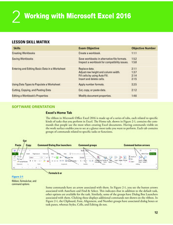
Page 2What is Excel?Excel is a spreadsheet program. A spreadsheet is a grid of rows and columns that helps organize, summarize,and calculate data. Spreadsheets are an everyday part of many professions, including accounting, statisticalanalysis, and project management. You can use Excel to create business forms, such as invoices and purchaseorders, among many other useful documents.This class teaches Microsoft Excel basics. To begin, let’s open Microsoft Excel. You can do this by clicking onStart, All Programs, Microsoft Office and Microsoft Excel. Let’s look at the toolbars.This is the Title Bar. It gives the name of the program and the title of the workbook you are using. Since wehave just opened up a new workbook and have not saved it with a name, the default title is Book1.On the left side of the Title bar is the Quick Access Toolbar.You can add or subtract commands to the toolbar by clicking on them inthe dropdown list that comes up by clicking.Under the Title Bar is the Ribbon. The Ribbon has eight Tabs that giveinstructions to the software. The Ribbon Tabs begin with File and continuewith Home, Insert, Page Layout, Formulas, Data, Review, and View. Onthe right-hand end, there is an icon for the Help Menu, Minimize, RestoreDown, and Close.Clicking on one of these tabs will open the Group. The Group that belongsto each tab shows related Command items together. You may then choose a Command.
Page 3Workbooks and WorksheetsWhen Excel is opened, a workbook appears with three worksheets. Each worksheet contains columns androws. There are 1,048,575 rows and 16,384 columns. The combination of a column coordinate and a rowcoordinate make up a cell address. For example, the cell located in the upper left corner of the worksheet iscell A1, meaning column A, row 1. The cell address is visible in the Name Box.Place your cursor in the first cell, A1. The formula bar will display the cell address in the Name Box on the leftside of the Formula Bar. Notice that the address changes as you move around the sheet. You can easily movefrom cell to cell by pressing tab or using the arrow keys.A cell can contain any of the following: A number (and any associated punctuation, such as decimal points, commas, and currency symbols).Text (including any combination of letters, numbers, and symbols that aren't number-related).A formula, which is a math equation.A function, which is a named equation that shortcuts an otherwise complex operation.Creating a New WorkbookIt is easy to create a new workbook! Simply, click on File – New and click on Blank Workbook to create a newworkbook.Creating a New WorksheetCreating a new worksheet is just as easy. By default, each Excel workbook contains three worksheets. Threetabs displaying Sheet 1, Sheet 2, and Sheet 3 will be displayed at the bottom of the workbook to indicate theseparate sheets. To add a new worksheet, simply click on the tab after the tab that says Sheet 3.Exercise 11. To change the location of a newly added worksheet, click once on the tab and hold down the leftmouse button and drag the worksheet to its new location.2. It is also possible to change the name of each worksheet. Right-click on the Sheet 1 tab and left-click onRename. Once you click on Rename, the name of the sheet becomes highlighted and you can simplytype in a new name. Double-clicking on the tab will also enable you to type in a new name.
Page 43. You can also change the color of the tabs by right-clicking on the tab and choosing Tab Color. Thensimply choose a color!!!4. It is possible to change the magnification of a worksheet so that you can read it better. To do this, clickon View and then Zoom. Go ahead and try the different magnifications to see which works best foryou. You can also make use of the Zoom bar in the lower right-hand corner to zoom to a comfortablereading size.Navigating and SelectingMoving around a worksheet is easy! You can easily move from cell to cell by using the arrow keys or pressingtab (will move the cursor to the right) or shift-tab (shift-tab will move you to the left). You can also use yourmouse to click within a cell which will select that cell. Sometimes you will want to select a range of cells.A range is a group of one or more cells. If you select more than one cell at a time, you can then performactions on the group of them at once, such as applying formatting or clearing the contents. A range can evenbe an entire worksheet.A range is referenced by the upper left and lower right cells. For example, the range of cells B1, B2, C1, and C2would be referred to as B1:C2.To select a range: With the mouse: Drag across the desired cells with the left mouse button held down. Be careful whenyou're positioning the mouse over the first cell (before pressing the mouse button). Position thepointer over the center of the cell, and not over an edge. You’ll know you are in the right spot whenyour cursor looks like this:If you drag while the pointer is on the edge of the cell, Excel interprets the selection as a move operationand whatever is in the cell(s) is dragged to a different spot. With the keyboard: Select the first cell, and then hold down the Shift key while you press the arrowkeys to expand the selection area.To select a nonrectangular or noncontiguous range, select the first portion of the range (that is, the firstrectangular piece), and then hold down the Ctrl key while you select additional cells/ranges with the mouse.
Page 5To select an entire column, click the column header (where the letter is). The cursor will be a vertical (forcolumns) or horizontal (for rows) black arrow. To select an entire row, click the row header (where thenumber is). You can click one row or column and then drag to select additional columns, or hold down Ctrl asyou click on the headers for noncontiguous rows and/or columns.Exercise 2Let’s practice:1. Click column B's letter to select that column.2. Hold Shift and click column D's letter. Columns B, C, and D should all be selected.3. Release the Shift key.4. Hold Ctrl and click column G's letter. Now B, C, D, and G are all selected.5. Release the Ctrl key.6. Press and hold the Shift key while pressing the down arrow key two times. Now B4 through B6 areselected. This range is called B4:B6.7. Still pressing the Shift key, press the right arrow two times. Now the range B4:D6 is selected.8. Press Ctrl A. This is a shortcut for selecting the entire sheet.9. Click in any cell to undo the selection.10. Click the square containing a gray triangle at the upper intersection of the column letters and the rownumbers. The entire sheet is selected again.Entering and Editing DataLet’s learn how to enter data into your worksheet. First, you place the cursor in the cell in which you wouldlike to enter data. Then you type the data and press Enter.Exercise 31. Place the cursor in cell A1.2. Type Jane. Tab to the next cell and type Smith.3. Move the cursor back to cell A1.4. Change Jane to Joe.
Page 6You can also edit information in a cell by double-clicking in a cell or by clicking in the formula bar. Trythese two options.Inserting Columns and RowsIf you don't plan your worksheet layout correctly, you might end up with too many or too few rows or columnsin a certain area. You can always move data around in the sheet to help with this, but sometimes it's easier tosimply insert or remove columns or rows.Exercise 4To insert a column or row:1. Right click on the column on the right of the two columns between which you wish to insert. (For example,if you wish to insert a column between E and F, right click on F.) If you wish to insert a row, right click onthe row’s number that is the one below where you wish to insert. (For example, if you wish to insert a rowbetween 3 and 4, right click on 4.)2. When the menu comes up, select Insert from the menu.Appearing to the left of your highlighted column or above your highlighted row will be a new row or column.Formatting Columns and RowsOften you will need to change your columns and rows in order for text to fit or for the text to fit on the pagecorrectly. There are a number of different methods one can use to do this. Let’s start with columns.Column Width: The formatting that is unique to columns is Column Width. Column Width is measuredin characters. A column's width can be from 0 to 255 characters, which is a really wide column! Decimal valuesare allowed. In fact, the default size is 8.43 characters.A width of 12, for example, means the column is wide enough for 12 average characters, using whatever youchose as the Standard font. The default is Calibri 11 pts. (To change the font from the default, go to ToolsOptions-General-Standard font).Column WidthExercise 5 – Autofit all
Page 71. Move your pointer to the right edge of the heading of Column A until it changes towhich is theResize Column shape.2. Press the left mouse button down. (Don't release it yet.)The popup tip appears, showing the currentwidth of Column A.3. Release the left mouse button and double-click in the same spot (the right edge of Column A'sheading). The column width changes so it is wide enough to display the longest text in any cell in thecolumn as a single line.Be careful when you set a column's width with AutoFit. The column may wind up wider than you expected.Any text will be on a single line in its cell. No matter how long the text is! If you accidentally find you'vewidened a cell out of sight to the right, use Undo. Then resize the column with another method.Column Width - DragDragging is a natural method of adjusting column width. But since you can't see the change until you releasethe mouse button, it may take you several attempts to get a satisfactory width.Exercise 61. Type in New Zealand in B1. Move the pointer to the right edge of column heading B.2. When the pointer changes to(the Resize Column shape), click and drag to the right until NewZealand shows entirely. Since the column is not resized until you release the mouse button, you mayneed several tries to get the width right.Row HeightT he only unique formatting for rows is Row Height. Row Height is measured in points, like font size, from 0 to409 points. A row height of zero hides the row.The default setting for Row Height is AutoFit. The row height adjusts to the largest font size in the row.AutoFit will leave a little white space, called the cell padding, between the text in the cell and the cell edges.When Calibri 11 pt. is the Standard Font, the Row Height is 15.00 points. Keep in mind that you can alwaysprint without the gridlines, which may make it look a little less crowded. That option is under Page Layout, inthe Sheet Options section.
Page 8Alignment OptionsWrapping TextWhen you enter text that is too long to fit in a cell into a cell, it overlaps the next cell. If you do not want it tooverlap the next cell you can wrap the text.Exercise 71.2.3.4.5.Open another new sheet.Move to cell A1.Type “Text too long to fit”. (After typing, click out of the cell and back in again.)From the Ribbon, choose Home Alignment Wrap Text.You will notice after you click Wrap Text, it is highlighted.Merging CellsSometimes, rather than having text wrap in a cell, you will actually want the text to run across the width of thedata. Usually when making a spreadsheet, you need to create a heading for the sheet. This heading should runacross the width of your data. To do this, one must merge the cells across the width of the data. Select therange of cells, and clickcentered over the data.the Merge and Center button under Alignment group. The heading is nowMoving to a New WorksheetIn Microsoft Excel, each workbook is made up of several worksheets. Before moving to the next topic, let’smove to a new worksheet. You can move from worksheet to worksheet by clicking on the tabs at the bottomof the worksheet. Let’s move to Sheet 2.Formatting Text and DataOnce information has been entered into a cell, you might want to change or enhance the way the informationis displayed. Text can be formatted in the same way that one uses in Microsoft Word or PowerPoint. Most ofthe formatting choices can be found in the Font grouping under the Home tab. There are numerous ways toformat data. Let’s look at some. Remember to always make sure that the cell you want to format is selected.Similar to Word, “if you want to affect it, you have to select it.”
Page 9Using Formatting ButtonsOn the Ribbon, make sure the Home tab is selected. In the Number Group box, there are several buttonswhich allow one-click formatting.From the dropdown box, you have several options – currency, percentage, date, and time and more.There are also buttons to increase decimal values, add a comma, or put in percentage.Notice how each number changes depending on the formatting.You can also format the cell by right clicking on the cell(s) and selecting the “Format Cells.” If the “Number”tab isn’t already selected, do so, and then select from the menu for currency, time, fraction, etc. Dependingon the option you choose, you will be given further options to the right.Exercise 81. Move the cursor to cell D1.2. Type 123456. Hit enter and then move back into D1. At this point it is necessary to move out of the celland then back in, as that is the only way to get the appropriate menu up!3. Right click on the number. A menu will pop up. Click on Format Cells.4. Click on “Number” tab at top, if necessary.5. Select “Currency” under Category and be sure that Decimal Places is set to 2.6. Click OK, and view the cell.It should look like the following:Deleting vs Clearing a Cell
P a g e 10Many beginners get confused about clearing versus deleting in Excel, so let's look at this concept briefly. Whenyou clear the content from a cell, the formatting for that cell is still there. It may be helpful to think of an Excelworksheet as a stack of empty cardboard boxes, each one with its open side facing you. You can putsomething into a cell or take something out. When you take something out of a cell, it's called clearing itscontent. The cell itself remains in the "stack," but it's now empty.To clear the content from a cell:1. Press Delete on the keyboard.2. Right-click the cell and then select Clear Contents.3. On the Home tab, in the Editing group, select Clear Clear Contents.Unfortunately, clearing a cell's content doesn't clear its formatting.To clear formatting:1. On the Home tab, in the Editing group, select Clear Clear Formats2. To clear both contents and formats at once, select Clear All.In contrast, deleting the cell removes the cell itself from the stack and makes the surrounding cells shift. Thinkabout what happens when you pull a box out of a stack of boxes -- the boxes above it fall down one position,right? It's the same thing with Excel cells, except it's reverse-gravity (cells fall up rather than down), and youhave the choice of making the remaining cells shift up or to the left. Let’s look at how this works.Filling Cells AutomaticallyYou can use Microsoft Excel to fill cells automatically with a series. For example, you can have Excelautomatically fill in times, the days of the week or months of the year, years, and other types of series. Days ofthe week and months of the year fill in a similar fashion.Exercise 91. Let’s move to another worksheet.2. In cell A1, type Sunday and click the B for bold in the Font group.3. Find the small black backward “L” in the lower right corner of the highlighted area. When you hoverover this backward “L,” the cursor will become a black “ .” This is called the Fill Handle.
P a g e 114. Grab the Fill Handle and drag with your mouse to fill cell A1 to G1. Note how the days of the week fillthe cells in a series. Also, note that the Auto Fill Options icon appears.5.6.7.8.Click the Auto Fill Options icon. Click on Copy Cells.Choose the Fill Series radio button. The cells fill as a series from Sunday to Saturday again.Click the Auto Fill Options icon again.Choose the Fill Without Formatting radio button. The cells fill as a series from Sunday to Saturday, but theentries are not bolded.9. Click the Auto Fill Options icon again.10. Choose the Fill Weekdays radio button. The cells fill as a series from Monday to Friday.Filling TimeExercise 101. Click on a new worksheet. Type 1:00 into cell A1.2. Grab the Fill Handle and drag with your mouse to highlight cells A1 to A24. Note that each cell fills using militarytime.3. Click anywhere on the worksheet to remove the highlighting.To change the format of the time:1.2.3.4.5.Select cells A1 to A24.Choose from the Ribbon: Home Number.Click on the drop down box and choose Time.The time is no longer in military time.If you wish to change the formatting further, click on the dropdown arrow in lower right-hand corner of numbergroup and choose the way you want the time to appear.Filling in Numbers
P a g e 12Exercise 111.2.3.4.Click on another worksheet. Type a 1 in cell A1.Grab the Fill Handle and drag with your mouse to highlight cells A1 to A7. The number 1 fills each cell.Click the Auto Fill Options icon.Choose the Fill Series radio button. The cells fill as a series starting with 1, 2, 3.And finally, here is one more interesting fill feature.1.2.3.4.Go to cell A1.Type Lesson 1.Grab the Fill Handle and drag with your mouse to highlight cells A1 to A6.The cells fill in as a series: Lesson 1, Lesson 2, Lesson 3, and so on.Performing Mathematical CalculationsFormulasA formula is an equation that performs some type of operation and issues a result. In Excel, formulas alwaysbegin with an equal sign. Here are some formula examples: 2 6: This formula is strictly math. If you place this formula in a cell, the cell displays 8. A1 6: Same as the preceding, but this time you're adding 6 to whichever value is in cell A1 and displaying theresult in the cell into which you enter this formula. This formula does not change A1's contents. A1 A2: Same thing again, but you're adding the contents of cell A1 to the contents of cell A2. A1 A2-A3: In this example, multiple cells are referenced.Here are the symbols you can use in formulas to indicate mathematical operations: : Addition-: Subtraction*: Multiplication/: DivisionExercise 12To try a basic formula, do the following:1. In a new worksheet, type 6 in cell A1 and 7 in cell A2.
P a g e 132. In cell A3, type A1 A2, and then press Enter.3. Select cell A3. Notice that it displays 13 in the cell itself, and in the formula bar, the original formula you enteredappears.4. Click in the formula bar to move the insertion point there and edit the formula to read as follows: A1 A2 5.Then press Enter. The value now appears as 18.5. Change the value in cell A1 to 4. The value in A3 changes to 16.AutosumLet’s add a column of numbers using the AutoSum ButtonEditing and automatically add a column of numbers. To select the AutoSum button choose Home Exercise 131. Type in the numbers 5, 7, 3, 9, 4, 8 in column C.2. Move your cursor to select C7. Click the AutoSum buttonEditing.3. C1 to C6 should now be highlighted.4. Press Enter. Cells C1 through C6 are added together.found on the Ribbon under Home You can also write a formula to sum a column by typing in: sum(c1:c6)Note that there is no space between sum and the parenthesis.More Formula ExamplesThe math operators in Excel have an order of operation, just like in regular math. The order of operation is the order inwhich they're processed when multiple operators appear in the same formula. Here are the rules that determine theorder:1. Any operations that are in parentheses, from left to right2. Multiplication (*) and division (/)3. Addition ( ) and subtraction (-)Parentheses override everything and go first. So, if you need to execute an operation out of the normal order, you placeit in parentheses. Now let's try some formula examples that refer to cells and use math operations. For this exercise,enter the following values in cells in a blank worksheet:
P a g e 14A1: 12 A2: 6A3: 4A4: 9Exercise 14Now let’s create the following formula:***In cell A5, create a formula that adds A1 A2 A3 A4.Preparing to PrintLet’s prepare to print! If your worksheet is more than one printed page, it is possible to have the heading oneach page by going to the Page Layout tab, in the Page Setup group and click Print Titles.On the Sheet tab, under Print Titles, do one or both of the following:
P a g e 15In the Rows to repeat at top box, type the reference of the rows that contain the column labels if youwant the heading repeated on each page.In the Columns to repeat at left box, type the reference of the columns that contain the row labels if youwant those to show.You can also click the Collapse Dialog button at the right end of the Rows to repeat at top andColumns to repeat at left boxes, and then select the title rows or columns that you want to repeat in theworksheet. After you finish selecting the title rows or columns, click the Collapse Dialog button againto return to the dialog box.We want our sheet to print with no gridlines, and centered horizontally across the page, but not vertically.We also want it to print in portrait orientation.1. Page tab: Make sure that Portrait is selected.2. Margins tab: All should be 0.5 inch. Click to Center on Page Horizontally.
P a g e 163. Sheet tab: There should not be a check under Print in the Gridline section.To print, click on File Print in the backstage area. Print preview automatically displays when you click onthe Print tab in the backstage view. Whenever you make a change to a print-related setting, the preview isautomatically updated. To view each page, click the arrows below the preview.Click the Print button toprint your document.Clicking the File tabdisplays the Backstagearea view.This dropdown showsthe currently selectedprinter. Clicking thedropdown will displayother availableprinters.These dropdown menus show currentlyClick the Print tab to print aselected Settings. Rather than justdocument, change print-showing you the name of a feature,related settings, and tothese dropdown menus show you whatautomatically display athe status of a feature is and describespreview of your document.it. This can help you figure out if youwant to change the setting from whatyou have.Make sure you take a look at the Preview Pane to assure that all of your columns and rows are showing. If all looks well,it’s now time to print!
P a g e 17Tips and TroubleshootingRecognizing Cursor StylesThere are four common cursor styles used in Excel.Click and drag tohighlight multiple cellswith this cursor, or clickin a cell to select thesingle cellClick and drag withthis cursor to fill cellcontents into cellsbelow or to the right.Click and drag the contents ofthe selected cell to any othercell.Click to place the cursorinto the Formula bar sothat you can edit anequation or function.Common formula errorsHere are some of the most common mistakes people make when entering formulas and functions: Not putting in all the required arguments: If a function is expecting more arguments than you haveentered, and you get a dialog box, be sure you've placed commas between the arguments and that youhaven't overlooked any. Circular references: If you refer to the cell's own address in a function, you create a circular error,which is like an endless loop. Suppose that you enter A1 1 into cell A1. You'll get an error messagelike the one below. If you click OK at this message, a Help window appears to help you find theproblem.
P a g e 18 Text in an argument: Most functions require numeric arguments. If you enter text as an argument, forexample, SUM(text), the word #NAME? appears in the cell. This happens because Excel allows you toname ranges of cells using text, so technically SUM(text) isn't an invalid function. It is invalid only ifthere's no range that has been assigned the name "text." Hash marks (###) in a cell: This happens when the cell isn't wide enough to display its value. Widen thecolumn to fix this.If you receive an error when copying a formula, don't panic; it happens to everyone. Use the skills you learnedearlier in this chapter to display the formulas and then check them for the common errors discussed here.Congratulations! You’ve completed the MS Excel 2010 Basics class. Please take a moment to fill out thesurvey. Your feedback is very important to us!
P a g e 5 To select an entire column, click the column header (where the letter is).The cursor will be a vertical (for columns) or horizontal (for rows) black arrow. To select an entire row, click the row header (where the number is). You can click one row or column and then drag to select additional columns, or hold down


