WIXLIB

186 Terrestrial uptake of CO2 is governed by net biome production (NBP), which is the balance of net primary production(NPP) and carbon losses due to heterotrophic respiration(decomposition and herbivory) and fire, including the fate ofharvested biomass. NPP increases when atmospheric CO2concentration is increased above present levels (the “fertilisation” effect occurs directly through enhanced photosynthesis, and indirectly through effects such as increasedwater use efficiency). At high CO2 concentration (800 to1,000 ppm) any further direct CO2 fertilisation effect is likelyto be small. The effectiveness of terrestrial uptake as a carbonsink depends on the transfer of carbon to forms with longresidence times (wood or modified soil organic matter).Management practices can enhance the carbon sink becauseof the inertia of these “slow” carbon pools.Feedbacks in the carbon cycle due to climate change Warming reduces the solubility of CO2 and therefore reducesuptake of CO2 by the ocean. Increased vertical stratification in the ocean is likely toaccompany increasing global temperature. The likelyconsequences include reduced outgassing of upwelled CO2,reduced transport of excess carbon to the deep ocean, andchanges in biological productivity. On short time-scales, warming increases the rate ofheterotrophic respiration on land, but the extent to which thiseffect can alter land-atmosphere fluxes over longer timescales is not yet clear. Warming, and regional changes inprecipitation patterns and cloudiness, are also likely to bringabout changes in terrestrial ecosystem structure, geographicdistribution and primary production. The net effect of climateon NBP depends on regional patterns of climate change.Other impacts on the carbon cycle Changes in management practices are very likely to havesignificant effects on the terrestrial carbon cycle. In additionto deforestation and afforestation/reforestation, more subtlemanagement effects can be important. For example, firesuppression (e.g., in savannas) reduces CO2 emissions fromburning, and encourages woody plant biomass to increase.On agricultural lands, some of the soil carbon lost when landwas cleared and tilled can be regained through adoption oflow-tillage agriculture. Anthropogenic N deposition is increasing terrestrial NPP insome regions; excess tropospheric ozone (O3) is likely to bereducing NPP. Anthropogenic inputs of nutrients to the oceans by rivers andatmospheric dust may influence marine biological productivity, although such effects are poorly quantified.Modelling and projection of CO2 concentrationProcess-based models of oceanic and terrestrial carbon cyclinghave been developed, compared and tested against in situmeasurements and atmospheric measurements. The followingare consistent results based on several models. Modelled ocean-atmosphere flux during 1980 to 1989 was inThe Carbon Cycle and Atmospheric Carbon Dioxidethe range 1.5 to 2.2 PgC/yr for the 1980s, consistent withearlier model estimates and consistent with the atmosphericbudget. Modelled land-atmosphere flux during 1980 to 1989 was inthe range 0.3 to 1.5 PgC/yr, consistent with or slightlymore negative than the land-atmosphere flux as indicated bythe atmospheric budget. CO2 fertilisation and anthropogenicN deposition effects contributed significantly: theircombined effect was estimated as 1.5 to 3.1 PgC/yr.Effects of climate change during the 1980s were small, andof uncertain sign. In future projections with ocean models, driven by CO2concentrations derived from the IS92a scenario (for illustration and comparison with earlier work), ocean uptakebecomes progressively larger towards the end of the century,but represents a smaller fraction of emissions than today.When climate change feedbacks are included, ocean uptakebecomes less in all models, when compared with thesituation without climate feedbacks. In analogous projections with terrestrial models, the rate ofuptake by the land due to CO2 fertilisation increases untilmid-century, but the models project smaller increases, or noincrease, after that time. When climate change feedbacks areincluded, land uptake becomes less in all models, whencompared with the situation without climate feedbacks.Some models have shown a rapid decline in carbon uptakeafter the mid-century.Two simplified, fast models (ISAM and Bern-CC) were used toproject future CO2 concentrations under IS92a and six SRESscenarios, and to project future emissions under five CO2stabilisation scenarios. Both models represent ocean andterrestrial climate feedbacks, in a way consistent with processbased models, and allow for uncertainties in climate sensitivityand in ocean and terrestrial responses to CO2 and climate. The reference case projections (which include climatefeedbacks) of both models under IS92a are, by coincidence,close to those made in the SAR (which neglected feedbacks). The SRES scenarios lead to divergent CO2 concentrationtrajectories. Among the six emissions scenarios considered,the projected range of CO2 concentrations at the end of thecentury is 550 to 970 ppm (ISAM model) or 540 to 960 ppm(Bern-CC model). Variations in climate sensitivity and ocean and terrestrialmodel responses add at least 10 to 30% uncertainty tothese values, and to the emissions implied by the stabilisationscenarios. The net effect of land and ocean climate feedbacks is alwaysto increase projected atmospheric CO2 concentrations. Thisis equivalent to reducing the allowable emissions for stabilisation at any one CO2 concentration. New studies with general circulation models includinginteractive land and ocean carbon cycle components alsoindicate that climate feedbacks have the potential to increaseatmospheric CO2 but with large uncertainty about themagnitude of the terrestrial biosphere feedback.

The Carbon Cycle and Atmospheric Carbon DioxideImplicationsCO2 emissions from fossil fuel burning are virtually certainto be the dominant factor determining CO2 concentrationsduring the 21st century. There is scope for land-use changesto increase or decrease CO2 concentrations on this time-scale.If all of the carbon so far released by land-use changes couldbe restored to the terrestrial biosphere, CO2 at the end of thecentury would be 40 to 70 ppm less than it would be if nosuch intervention had occurred. By comparison, globaldeforestation would add two to four times more CO2 to theatmosphere than reforestation of all cleared areas wouldsubtract.3.1 IntroductionThe concentration of CO2 in the atmosphere has risen from closeto 280 parts per million (ppm) in 1800, at first slowly and thenprogressively faster to a value of 367 ppm in 1999, echoing theincreasing pace of global agricultural and industrial development. This is known from numerous, well-replicated measurements of the composition of air bubbles trapped in Antarctic ice.Atmospheric CO2 concentrations have been measured directlywith high precision since 1957; these measurements agree withice-core measurements, and show a continuation of theincreasing trend up to the present.Several additional lines of evidence confirm that the recentand continuing increase of atmospheric CO2 content is causedby anthropogenic CO2 emissions – most importantly fossil fuelburning. First, atmospheric O2 is declining at a rate comparablewith fossil fuel emissions of CO2 (combustion consumes O2).Second, the characteristic isotopic signatures of fossil fuel (itslack of 14C, and depleted content of 13C) leave their mark in theatmosphere. Third, the increase in observed CO2 concentrationhas been faster in the northern hemisphere, where most fossilfuel burning occurs.Atmospheric CO2 is, however, increasing only at about halfthe rate of fossil fuel emissions; the rest of the CO2 emittedeither dissolves in sea water and mixes into the deep ocean, or istaken up by terrestrial ecosystems. Uptake by terrestrial ecosystems is due to an excess of primary production (photosynthesis)over respiration and other oxidative processes (decomposition orcombustion of organic material). Terrestrial systems are also an187There is sufficient uptake capacity in the ocean to incorporate70 to 80% of foreseeable anthropogenic CO2 emissions to theatmosphere, this process takes centuries due to the rate of oceanmixing. As a result, even several centuries after emissionsoccurred, about a quarter of the increase in concentration causedby these emissions is still present in the atmosphere.CO2 stabilisation at 450, 650 or 1,000 ppm would requireglobal anthropogenic CO2 emissions to drop below 1990 levels,within a few decades, about a century, or about two centuriesrespectively, and continue to steadily decrease thereafter.Stabilisation requires that net anthropogenic CO2 emissionsultimately decline to the level of persistent natural land and oceansinks, which are expected to be small ( 0.2 PgC/yr).anthropogenic source of CO2 when land-use changes (particularly deforestation) lead to loss of carbon from plants and soils.Nonetheless, the global balance in terrestrial systems is currentlya net uptake of CO2.The part of fossil fuel CO2 that is taken up by the ocean andthe part that is taken up by the land can be calculated from thechanges in atmospheric CO2 and O2 content because terrestrialprocesses of CO2 exchange involve exchange of oxygen whereasdissolution in the ocean does not. Global carbon budgets basedon CO2 and O2 measurements for the 1980s and 1990s areshown in Table 3.1. The human influence on the fluxes of carbonamong the three “reservoirs” (atmosphere, ocean, and terrestrialbiosphere) represent a small but significant perturbation of ahuge global cycle (Figure 3.1).This chapter summarises current knowledge of the globalcarbon cycle, with special reference to the fate of fossil fuel CO2and the factors that influence the uptake or release of CO2 by theoceans and land. These factors include atmospheric CO2 concentration itself, the naturally variable climate, likely climate changescaused by increasing CO2 and other greenhouse gases, changes inocean circulation and biology, fertilising effects of atmosphericCO2 and nitrogen deposition, and direct human actions such asland conversion (from native vegetation to agriculture and viceversa), fire suppression and land management for carbon storageas provided for by the Kyoto Protocol (IPCC, 2000a). Anychanges in the function of either the terrestrial biosphere or theocean whether intended or not could potentially have significant effects, manifested within years to decades, on the fraction offossil fuel CO2 that stays in the atmosphere. This perspective has

0.4Rockcarbonates902–lysocline3,500 mthermocline100 DOC/POC110.2dissolution0.7export ofsoft tissueCaCO3900.40.2CaCO3export ofCaCO 0]heterotrophic respiration 34autotrophic respiration 58NPPGPPspirphic re33 physicaltransportDIC in surface waterCO2 H 2 O CO388c) Carbon cycling in the oceanriver transport0.8weathering0.2120weathering0.2DOC export 0.4GEOLOGICALRESERVOIRSFossilorganiccarbonLANDSoil Plants[1500] [500]0.4vulcanism 0.1a) Main components of the natural carbon cycle10.?4'INERT'CARBON 1000yr[150] dMODIFIEDSOIL CARBON 10 to 1000yr[1050]LANDDOCexport0.4d) Carbon cycling on OIRSFossilorganiccarbonsfosinurnlbeil fu.3g5b) The human perturbationge1.Animalsocean totrophicrespiration60DETRITUS 10yr[300]7ATMOSPHERE188The Carbon Cycle and Atmospheric Carbon Dioxide

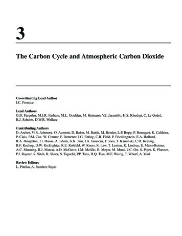
The Carbon Cycle and Atmospheric Carbon Dioxidedriven a great deal of research during the years since the IPCCWGI Second Assessment report (IPCC, 1996) (hereafter SAR)(Schimel et al., 1996; Melillo et al., 1996; Denman et al., 1996).Some major areas where advances have been made since the SARare as follows: Observational research (atmospheric, marine and terrestrial)aimed at a better quantification of carbon fluxes on local,regional and global scales. For example, improved precision andrepeatability in atmospheric CO2 and stable isotope measurements; the development of highly precise methods to measurechanges in atmospheric O2 concentrations; local terrestrial CO2flux measurements from towers, which are now beingperformed continuously in many terrestrial ecosystems; satelliteobservations of global land cover and change; and enhancedmonitoring of geographical, seasonal and interannual variationsof biogeochemical parameters in the sea, including measurements of the partial pressure of CO2 (pCO2) in surface waters. Experimental manipulations, for example: laboratory andgreenhouse experiments with raised and lowered CO2 concentrations; field experiments on ecosystems using free-air carbondioxide enrichment (FACE) and open-top chamber studies ofraised CO2 effects, studies of soil warming and nutrient enrichment effects; and in situ fertilisation experiments on marineecosystems and associated pCO2 measurements.189 Theory and modelling, especially applications of atmospherictransport models to link atmospheric observations to surfacefluxes (inverse modelling); the development of process-basedmodels of terrestrial and marine carbon cycling andprogrammes to compare and test these models against observations; and the use of such models to project climate feedbackson the uptake of CO2 by the oceans and land.As a result of this research, there is now a more firmly basedknowledge of several central features of the carbon cycle. Forexample: Time series of atmospheric CO2, O2 and 13CO2 measurementshave made it possible to observationally constrain thepartitioning of CO2 between terrestrial and oceanic uptake andto confirm earlier budgets, which were partly based on modelresults. In situ experiments have explored the nature and extent of CO2responses in a variety of terrestrial ecosystems (includingforests), and have confirmed the existence of iron limitations onmarine productivity. Process-based models of terrestrial and marine biogeochemicalprocesses have been used to represent a complex array offeedbacks in the carbon cycle, allowing the net effects of theseprocesses to be estimated for the recent past and for futurescenarios.Figure 3.1: The global carbon cycle: storages (PgC) and fluxes (PgC/yr) estimated for the 1980s. (a) Main components of the natural cycle. Thethick arrows denote the most important fluxes from the point of view of the contemporary CO2 balance of the atmosphere: gross primary production and respiration by the land biosphere, and physical air-sea exchange. These fluxes are approximately balanced each year, but imbalances canaffect atmospheric CO2 concentration significantly over years to centuries. The thin arrows denote additional natural fluxes (dashed lines forfluxes of carbon as CaCO3), which are important on longer time-scales. The flux of 0.4 PgC/yr from atmospheric CO2 via plants to inert soilcarbon is approximately balanced on a time-scale of several millenia by export of dissolved organic carbon (DOC) in rivers (Schlesinger, 1990). Afurther 0.4 PgC/yr flux of dissolved inorganic carbon (DIC) is derived from the weathering of CaCO3, which takes up CO2 from the atmosphere ina 1:1 ratio. These fluxes of DOC and DIC together comprise the river transport of 0.8 PgC/yr. In the ocean, the DOC from rivers is respired andreleased to the atmosphere, while CaCO3 production by marine organisms results in half of the DIC from rivers being returned to the atmosphereand half being buried in deep-sea sediments which are the precursor of carbonate rocks. Also shown are processes with even longer time-scales:burial of organic matter as fossil organic carbon (including fossil fuels), and outgassing of CO2 through tectonic processes (vulcanism). Emissionsdue to vulcanism are estimated as 0.02 to 0.05 PgC/yr (Williams et al., 1992; Bickle, 1994). (b) The human perturbation (data from Table 3.1).Fossil fuel burning and land-use change are the main anthropogenic processes that release CO2 to the atmosphere. Only a part of this CO2 stays inthe atmosphere; the rest is taken up by the land (plants and soil) or by the ocean. These uptake components represent imbalances in the largenatural two-way fluxes between atmosphere and ocean and between atmosphere and land. (c) Carbon cycling in the ocean. CO2 that dissolves inthe ocean is found in three main forms (CO2, CO32 , HCO3 , the sum of which is DIC). DIC is transported in the ocean by physical and biologicalprocesses. Gross primary production (GPP) is the total amount of organic carbon produced by photosynthesis (estimate from Bender et al., 1994);net primary production (NPP) is what is what remains after autotrophic respiration, i.e., respiration by photosynthetic organisms (estimate fromFalkowski et al., 1998). Sinking of DOC and particulate organic matter (POC) of biological origin results in a downward flux known as exportproduction (estimate from Schlitzer, 2000). This organic matter is tranported and respired by non-photosynthetic organisms (heterotrophic respiration) and ultimately upwelled and returned to the atmosphere. Only a tiny fraction is buried in deep-sea sediments. Export of CaCO3 to the deepocean is a smaller flux than total export production (0.4 PgC/yr) but about half of this carbon is buried as CaCO3 in sediments; the other half isdissolved at depth, and joins the pool of DIC (Milliman, 1993). Also shown are approximate fluxes for the shorter-term burial of organic carbonand CaCO3 in coastal sediments and the re-dissolution of a part of the buried CaCO3 from these sediments. (d) Carbon cycling on land. Bycontrast with the ocean, most carbon cycling through the land takes place locally within ecosystems. About half of GPP is respired by plants. Theremainer (NPP) is approximately balanced by heterotrophic respiration with a smaller component of direct oxidation in fires (combustion).Through senescence of plant tissues, most of NPP joins the detritus pool; some detritus decomposes (i.e., is respired and returned to theatmosphere as CO2) quickly while some is converted to modified soil carbon, which decomposes more slowly. The small fraction of modified soilcarbon that is further converted to compounds resistant to decomposition, and the small amount of black carbon produced in fires, constitute the“inert” carbon pool. It is likely that biological processes also consume much of the “inert” carbon as well but little is currently known about theseprocesses. Estimates for soil carbon amounts are from Batjes (1996) and partitioning from Schimel et al. (1994) and Falloon et al. (1998). Theestimate for the combustion flux is from Scholes and Andreae (2000). ‘τ’ denotes the turnover time for different components of soil organic matter.

190The Carbon Cycle and Atmospheric Carbon DioxideBox 3.1: Measuring terrestrial carbon stocks and fluxes.Estimating the carbon stocks in terrestrial ecosystems and accounting for changes in these stocks requires adequate informationon land cover, carbon density in vegetation and soils, and the fate of carbon (burning, removals, decomposition). Accounting forchanges in all carbon stocks in all areas would yield the net carbon exchange between terrestrial ecosystems and the atmosphere(NBP).Global land cover maps show poor agreement due to different definitions of cover types and inconsistent sources of data (deFries and Townshend, 1994). Land cover changes are difficult to document, uncertainties are large, and historical data are sparse.Satellite imagery is a valuable tool for estimating land cover, despite problems with cloud cover, changes at fine spatial scales,and interpretation (for example, difficulties in distinguishing primary and secondary forest). Aerial photography and groundmeasurements can be used to validate satellite-based observations.The carbon density of vegetation and soils has been measured in numerous ecological field studies that have been aggregatedto a global scale to assess carbon stocks and NPP (e.g., Atjay et al., 1979; Olson et al., 1983; Saugier and Roy, 2001; Table 3.2),although high spatial and temporal heterogeneity and methodological differences introduce large uncertainties. Land inventorystudies tend to measure the carbon stocks in vegetation and soils over larger areas and/or longer time periods. For example, theUnited Nations Food and Agri

The Carbon Cycle and Atmospheric Carbon Dioxide 185 Executive Summary CO 2 concentration trends and budgets Before the Industrial Era, circa 1750, atmospheric carbon dioxide (CO 2) concentration was 280 10 ppm for several thousand years. It has