Transcription
This is a preprint of the following article:Shamsheer S. Chauhan and J. R. R. A. Martins. Tilt-wing eVTOL takeoff trajectory optimization. Journal of Aircraft, 2019.The published article may differ from this preprint and is available at:https://doi.org/10.2514/1.C035476.Tilt-wing eVTOL takeoff trajectoryoptimizationShamsheer S. Chauhan and Joaquim R. R. A. MartinsUniversity of Michigan, Ann Arbor, MI, 48109AbstractTechnological advances in areas such as battery technology, autonomous control, andride-hailing services, combined with the scale-free nature of electric motors, havesparked significant interest in electric vertical takeoff and landing (eVTOL) aircraftfor urban air mobility. In this work, we use simplified models for the aerodynamics,propulsion, propeller-wing flow interaction, and flight mechanics to carry out gradientbased optimization studies for the takeoff-to-cruise trajectory of a tandem tilt-wingeVTOL aircraft. We present results for optimizations with and without stall and acceleration constraints, with varying levels of flow augmentation from propellers, andfind that the optimal takeoffs involve stalling the wings or flying near the stall angleof attack. However, we find that the energy penalty for avoiding stall is practicallynegligible. Additionally, we find that without acceleration constraints, the optimizedtrajectories involve rapidly transitioning to forward flight and accelerating, followedby climbing at roughly constant speed, and then accelerating to the required cruisespeed. With an acceleration constraint for passenger comfort, the transition, climb,and acceleration phases are more gradual and less distinct. We also present resultsshowing the impact of wing loading and available power on the optimized trajectories.1IntroductionThe fundamentally different nature of electric motors, compared to combustion engines, allows developing unconventional aircraft configurations that would otherwisebe impractical. This, combined with advances in battery technology, autonomous control, and ride-hailing services, makes large-scale urban air transportation seem morefeasible than ever. This possibility of urban air transportation is currently receivingsignificant interest and a large number of different electric vertical takeoff and landing(eVTOL) aircraft are currently under development. A few examples of the companies currently developing passenger eVTOL aircraft are Airbus, Aurora Flight Sciences1
(a Boeing subsidiary), EHang, Joby Aviation, Kitty Hawk, Lilium, and Volocopter.Most of the concepts under development can be categorized into a few major categories of aircraft type. Four of these major categories are multicopter (e.g., Volocopter2X), lift cruise (e.g., Kitty Hawk Cora), tilt-rotor (e.g., Joby S4), and tilt-wing (e.g.,Airbus A3 Vahana) [1].An eVTOL aircraft currently being developed by Airbus A3 , called the Vahana, hasa tandem tilt-wing configuration. This type of aircraft has tilting wings with propellerson them that allow the aircraft to takeoff and land vertically like a helicopter, but cruiselike an airplane. This configuration is one of the many solutions that allow achievingboth the takeoff and landing flexibility of helicopters, and the efficient forward flightof airplanes.Tilt-wing aircraft first received serious attention in the 1950s and 1960s when a fewcompanies including Boeing, Ling-Temco-Vought (LTV), Hiller, and Canadair developed flying prototype aircraft [2–8]. Several successful flight tests including transitionsbetween vertical and horizontal flight were carried out [2–5, 7]. Flight-test summariesfor the Boeing-Vertol VZ-2 [2] and Canadair CL-84 [5] report that flow separation andstalling of the wings provided piloting and operational challenges. Over 300 hours offlight testing was carried out for the LTV/Hiller/Ryan XC-142 to prove its suitability for operation [4]. Despite the extensive testing, due to several factors includingchallenges related to control and stability as well as mechanical complexity, interestwas lost and these programs were eventually canceled. However, with modern controlsystems and the advantages of electric propulsion, modern tilt-wing concepts may beable to overcome these challenges. A significant amount of literature also exists fromthat period related to the design, performance, and control of tilt-wing aircraft [9–14].More recent work has focused on the design and control of smaller tilt-wing unmannedaerial vehicles (UAVs) [15–19].Transitioning from vertical to horizontal flight for a tilt-wing aircraft is a balancingact in which the propellers have to provide sufficient thrust to support the weight ofthe aircraft while also tilting with the wings to accelerate the aircraft to a speed andconfiguration where sufficient lift can be provided by the wings. This transition isan important consideration for the design of these types of aircraft. Separated flowover the wing, which is undesirable and avoided in conventional aircraft design, is animportant concern during the transition for tilt-wing aircraft and may even be beneficialor unavoidable. Johnson et al. [1] briefly mention in their conference paper that theiranalysis for a tilt-wing eVTOL concept suggests that the wing is operating near orjust beyond stall during transition. Based on testing for the NASA Greased LightningGL-10 prototypes, it also seems possible that spending some time with the wing stalledmay provide the most energy-efficient transition for a tilt-wing aircraft [19].Stalling the wing during the transition process allows prioritizing acceleration andtransitioning to the more efficient airplane configuration more quickly at the cost ofsome inefficient lift during early stages. However, it is not obvious whether this providesan overall benefit. Also, if it does, it is not obvious how much of a benefit it provides.One of our goals in this paper is to investigate this further for a tandem tilt-wingpassenger eVTOL configuration based on the Airbus A3 Vahana.There is a lack of studies on the optimal takeoff trajectory for passenger tilt-wing2
eVTOL aircraft. However, some related research has been carried out on transition optimization for tailsitter and flying-wing UAVs that take off vertically. Stone and Clarke[20] carried out numerical optimization studies for the takeoff maneuver of a 23–32 kgtailsitter twin-propeller wing-canard UAV with the objective of minimizing the timerequired to transition to forward flight and reach a specified altitude and speed. Theylimit the angles of attack in their optimization problem to prevent stalling the wingand conclude that it is possible for their UAV to transition without stalling the wing.They also note that as aircraft mass increases, the optimal takeoff maneuvers haveincreased angles of attack for greater portions of the maneuver. Another interestingobservation from their results is that for larger aircraft masses, the optimal takeofftrajectory involves overshooting the target altitude and then descending to achieve it.In a later paper, Stone et al. [21] also discuss flight-test results for their UAV and notethat during the vertical to forward-flight transition, the UAV lost altitude instead ofgaining altitude as predicted by their simulations.Kubo and Suzuki [22] numerically optimized the transitions between hover andforward flight for a 2 kg tailsitter UAV with a twin-propeller twin-boom wing-tail configuration. With the objective of minimizing transition time, and with stall constraints,they obtain an optimized transition from hover to forward flight without noticeable altitude change. They also note that high throttle settings during the transition helpdelay stall.Maqsood and Go [23] numerically optimized transitions between hover and cruisefor a small tailsitter tilt-wing UAV (tractor configuration without distributed propulsion) with the objective of minimizing the altitude variation during transition. Theycompare optimization results for the hover to forward-flight transition for a configuration with tilting wings and the same configuration with fixed wings. They note thatthe optimal transition with a tilting wing avoids stalling the wing, which reduces thrustrequirements compared to a fixed-wing configuration.Oosedo et al. [24] numerically optimized the hover to forward-flight transition for a3.6 kg quadrotor tailsitter flying-wing UAV with the objective of minimizing the timerequired to transition. They compare optimization cases with and without constraintsfor maintaining altitude. They also compare their simulations to experimental flighttests. All four of the UAVs [20, 22–24] mentioned above are significantly different fromthe type of aircraft we are interested in, due to their configurations and sizes.Two other related research efforts focus on the landing phase instead. Pradeepand Wei [25] optimized the speed profile and time spent in the cruise, deceleration-tohover, hover, and descent phases given a fixed arrival time requirement for the AirbusA3 Vahana configuration. However, they do not model or study the details of thetransition from cruise to hover. Verling et al. [26] optimized the transition from cruiseto hover for a 3 kg tail-sitter flying-wing UAV.For all the optimization studies mentioned above, relatively low-order models areused for the multiple disciplines involved due to the complexity of the physics andthe high computational cost of higher-order methods. For the aerodynamics, the approaches used by these studies include using a database with aerodynamic coefficientsand derivatives from a panel method [20], using airfoil data with corrections [22], andinterpolating wind-tunnel data [23, 24, 26]. For propulsion, these studies either use3
momentum theory and variations of blade-element models [20, 22] or experimentaldata [24]. For the propeller-wing interaction, all of the above studies that considerit augment the flow over the wing using induced-velocity estimates based on momentum theory [22, 23, 26], except for Stone and Clarke [20] who connect a blade-elementmodel to a panel-method model and account for both axial and tangential inducedvelocities [27]. For the flight dynamics, representing the aircraft using a three degreesof-freedom (DOF) longitudinal model is the common approach [20, 22–24, 26].To address the lack of literature on the optimal takeoff trajectory for passengertilt-wing eVTOL aircraft, we present numerical optimization results for the takeoffto-cruise phase of a tandem tilt-wing eVTOL configuration based on the Airbus A3Vahana. The optimization objective is to minimize the electrical energy required toreach a specified cruise altitude and speed. In this paper, we answer the followingquestions:1. What does the optimal takeoff trajectory including transition and climb (to acruise altitude and speed appropriate for air-taxi operations) look like?2. Does the optimal trajectory involve stalling the wings and, if yes, how much of abenefit does it provide?3. How does the augmented flow over the wings due to propellers affect the optimaltrajectory and energy consumption?4. How much electrical energy is required?5. How does the wing loading affect the optimal trajectory?6. How does the power-to-weight ratio affect the optimal trajectory?We use simplified models, gradient-based optimization, and NASA’s OpenMDAO framework [28, 29] (a Python-based open-source optimization framework) for the optimizations.By “simplified” models we mean computationally inexpensive first-principles-basedlow-order models that capture the primary trends. To model the aerodynamics of thewings we use a combination of airfoil data, well-known relations from lifting-line theory,and the post-stall model developed by Tangler and Ostowari [30]. For the propulsionand propeller-wing interaction we use relations from momentum theory and bladeelement theory. For the flight mechanics we use a simplified 2-DOF representation ofthe aircraft and the forward Euler method for time integration.This paper is organized as follows. In Section 2 we describe the mathematicalmodels used in this work. In Section 3 we describe the optimization problems. Finally,in Section 4, we present and discuss the optimization results.2Mathematical modelsWe use the simplified models for the aerodynamics, propulsion, propeller-wing interaction, and flight-mechanics disciplines as described in the rest of this section. Asmentioned earlier, by “simplified” models we mean computationally inexpensive firstprinciples-based low-order models that capture the primary trends.4
2.1AerodynamicsFigure 1 shows the side view of the aircraft configuration that we use for this work. Itis a tandem tilt-wing configuration based on the Airbus A3 Vahana. The configurationhas two rectangular tilting wings, each with four propellers in front. The total wingplanform area is 9 m2 , an estimate based on online images of an Airbus A3 Vahanafull-scale flight-test prototype. For the configuration we model, we assume that theforward and rear wings are identical and have the same reference area for simplicity.However, note that the actual Airbus A3 Vahana prototype has a smaller forward wing(approximately 20% smaller than the rear wing based on flight-test prototype images).Rear propellersRear wingForward propellersFuselageForward wingFigure 1: Side view of the VTOL configuration of interest. The configuration has tworectangular tilting wings.Since separated-flow conditions need to be considered for the transition from verticalto horizontal flight, we require a model for the aerodynamics of the wings that alsopredicts the lift and drag beyond the linear-lift region. We use a model developedby Tangler and Ostowari [30] for non-rotating finite-length rectangular wings basedon experimental data and the model of Viterna and Corrigan [31]. The post-stall liftcoefficient is given bycos2 α,(1)CL A1 sin 2α A2sin αwhereC1A1 ,(2)2sin αs,(3)A2 (CLs C1 sin αs cos αs )cos2 αsandC1 1.1 0.018AR.(4)Here, α is the wing angle of attack, αs is the angle of attack at stall, CLs is the liftcoefficient at stall, and AR is the wing aspect ratio. Before stall, the airfoil lift anddrag are modified using the well-known finite-wing corrections from lifting-line theoryfor unswept wings in incompressible flow.5
Between 27.5 and 90 , the drag coefficient is given by:CD B1 sin α B2 cos α,(5)B1 CDmax ,(6)CDs CDmax sin αs,cos αs(7)1.0 0.065AR.0.9 t/c(8)whereB2 andCDmax Here CDs is the drag coefficient at stall and t/c is the airfoil thickness-to-chord ratio.For the post-stall drag coefficient below 27.5 , the data points listed in Table 1 areused.Table 1: Post-stall drag coefficient data points below 27.5 from Tangler and Ostowari[30]αCD 160.10020 0.17525 0.27527.5 0.363Viterna and Corrigan [31] and Tangler and Ostowari [30] note that post-stall characteristics are relatively independent of airfoil geometry, which is why we do not seeany input directly related to camber in the above equations. Tangler and Ostowari[30] also note that post-stall characteristics are relatively independent of the Reynoldsnumber in the high-Reynolds range. Tangler and Ostowari [30] based their modifications to the Viterna and Corrigan [31] model on finite-length fixed-wing experimentaldata from Ostowari and Naik [32] who conducted tests at Reynolds numbers rangingfrom 0.25 million to 1 million. This also happens to be a reasonable Reynolds numberrange for the takeoff phase of the configuration we are looking at. The advantage ofthis model is that it provides reasonable predictions that can be evaluated at very littlecomputational cost. In Appendix A, we have included plots that compare the aboveTangler–Ostowari model to finite-wing experimental data from Ostowari and Naik [32]for NACA 4415 and NACA 4412 wings of different aspect ratio and with differentReynolds numbers.For the airfoil used by the configuration of interest, we assume the NACA 0012symmetric airfoil for simplicity. For the pre-stall aerodynamics, we refer to NACA 0012experimental data from Critzos et al. [33] and Abbott and Von Doenhoff [34]. Weestimated the lift-curve slope from the experimental data collected by Critzos et al.6
[33] (smooth airfoil at Re 1.8 · 106 ) as 5.9 rad 1 and correct it using the followingwell-known correction for finite wings based on lifting-line theory:awing aairfoil,airfoil1 aπARe(9)where awing is the finite-wing lift-curve slope, aairfoil is the airfoil lift-curve slope, and eis the span efficiency factor. We assume that the pre-stall lift curve is linear and thatthe stall angle of attack of the wing is 15 .For each wing’s parasite drag before stall, we use airfoil drag coefficient values fromthe NACA 0012 drag polar provided by Abbott and Von Doenhoff [34] (smooth airfoilat Re 3 · 106 ). The data points we use are listed in Table 5 in Appendix B undercd . To obtain these cd values from the drag polar, we first related α to the sectionallift coefficient, cl . This was done using cl α · aairfoil . Using this relation is notstrictly correct because the sectional lift coefficient will vary across the wing. However,this gives a reasonable and conservative estimate. To these pre-stall parasite dragcoefficients, we add induced drag using the well-known formula based on lifting-linetheory,CL2,(10)CDi πAReto obtain the total drag of the wing before stall. Here CDi is the induced drag coefficient,CL is the wing’s lift coefficient, and for our configuration AR 8 for each wing.For simplicity, we compute the lift and drag of each wing in the tandem configuration as if they are independent and isolated wings. However, since we have a tandemconfiguration, we consider some interaction to determine the equivalent span efficiency,e, for each wing to avoid underpredicting drag. Based on the classical work of Munkand Prandtl [35], the induced drag of a biplane configuration with two identical wingsgenerating the same amount of lift, Lper wing , is 2 Lper wingL2per wing12 2σ,(11)Dinduced πqb2b2where q is the freestream dynamic pressure, b is the span, and σ is a factor for theinterference between the wings. This assumes that the two wings have elliptical liftdistributions. For an equal-span tandem configuration with an effective gap-to-spanratio of 0.25, σ is approximately 0.4 [36].For our configuration, we assume that with the effects of having a propeller at thewingtips, we can obtain a high span efficiency of approximately 0.95 for each wing inisolation. If we assume an effective gap-to-span ratio of 0.25 (i.e., σ 0.4), and assumethat Eq. (11) is valid for the assumed high span efficiency of 0.95, the induced drag forthe configuration is 2 L2per wingLper wingDinduced 2 1.4 2.(12)πqb2 · 0.95πqb2 · 0.68This means that when modeling the biplane as two isolated wings, the effective spanefficiency, e, for each wing is approximately 0.68 (i.e., 0.95/1.4). We use this value of e7
in Eq. (10) for our computations (computing the lift and drag of each wing as if theywere isolated).Since the Tangler–Ostowari model [30] described earlier only provides an analyticequation for the drag coefficient beyond 27.5 , we also desire an equation for the dragcoefficient below this angle. To obtain an equation for the drag coefficient below 27.5 ,we fit a quartic polynomial to the CD values in Table 5 and Table 1 to obtainCD 0.008 1.107α2 1.792α4 ,(13)which is a least-squares fit where α is in radians. This curve and the data points areplotted in Fig. 16 in Appendix B.The resulting lift and drag curves for each rectangular wing with AR 8 using theTangler–Ostowari [30] model are shown in Fig. 2. Since the curves shown in Fig. 2 havepoints at which the slopes are discontinuous, we use Kreisselmeier–Steinhauser (KS)functions [37] to make them C1 continuous for gradient-based optimization. Figure 3shows the regions of the lift and drag curves that are C1 discontinuous and comparesthem to the curves from the KS functions that are used to smooth 50.00153045α[ ]60750.0090(a) Lift coefficient0153045α [ ]607590(b) Drag coefficientFigure 2: Finite-wing (AR 8) coefficients of lift and drag using the Tangler–OstowarimodelWe must also note that for low flight speeds at the beginning of takeoff, especiallyfor the cases where there is no flow over the wings from the propellers, the errors ofthis model may be significant due to the different behavior of flow at low Reynoldsnumbers [38].This approach for modeling the aerodynamics of the wings is similar in nature tothe approach used by Kubo and Suzuki [22], who use airfoil data that includes poststall angles ( 180 to 180 ). However, it is not clear how they correct the airfoil datafor finite-wing effects. As mentioned in the introduction, the other approaches used instudies similar to this work include using a database with aerodynamic coefficients andderivatives from a panel method [20] and interpolating wind-tunnel data [23, 24, 26].8
.4KSKS1.00.151015α [ ]20253015(a) Comparing the C1 -discontinuous partof the lift coefficient curve and the smoothKS function curve2025α [ ]303540(b) Comparing the C1 -discontinuous partof the drag coefficient curve and thesmooth KS function curveFigure 3: Comparison of the C1 -discontinuous lift and drag coefficient curves to smoothcurves obtained using KS functionsWe have not come across the use of the Tangler–Ostowari [30] model in researchrelated to airplane performance and design. However, this is not surprising becausethese relations are for the post-stall behavior of rectangular wings. Airplane performance and design usually does not require modeling post-stall behavior, and for thecases that do, the wings are usually not rectangular or in uniform freestream flow. Theadvantage of using the approach described here, over methods such as panel methodsand RANS-based CFD, is that it provides reasonable predictions at very low cost dueto the use of analytical equations. Additionally, obtaining accurate stall and post-stallpredictions with higher-order methods such as panel methods and RANS-based CFDis a major challenge [39–44].To the drag computed for the wings using the equations described above, we furtheradd drag based on an assumed drag area of 0.35 for the fuselage and fixed landing gear,which is the value used in the open-source trade-studies code1 shared by the Airbus A3Vahana team. We also assume that this coefficient for the fuselage and landing gear isindependent of the freestream angle of attack and that the fuselage does not contributeany additional lift apart from the lift computed for the portions of the wing planformsthat overlap with the fuselage.As discussed earlier, we assume that both of the wings in our tandem configurationare identical. Apart from the interaction considered when computing the effectivespan efficiency for each wing, we assume that there is no interaction of flow betweenthe two wings. We also assume that the two wings rotate identically, so this meansthat the angles of attack seen by the two wings are assumed to be identical, and soare the lift and drag that they generate. Additionally, we assume that the wings eStudy[Accessed: Dec 2018]9
located forward and aft of the center of gravity (CG) such that their moments arealways balanced and ignore any fine-tuning required for trim and stability. In reality,even with symmetric airfoils and identical vertically offset wings located with theirquarter-chords equidistant from the CG, the forces and moments on the wings willnot be identical and the aircraft will not stay perfectly balanced due to several factorsincluding upwash and downwash, propeller interactions, CG movement, and fuselagemoments. However, we assume their effects to be small and also neglect the effects ofany rotation caused by them on the forces on the aircraft.2.2PropulsionTo compute thrust from the propellers as a function of power, we use the followingrelation based on momentum theory: s2V T V ,(14)Pdisk T V κT 242ρAdiskwhere Pdisk is the power supplied to the propeller disk excluding profile power, T isthe thrust, V is the component of the freestream velocity normal to the propellerdisk, ρ is the air density, Adisk is the disk area of the propeller, and κ is a correctionfactor to account for induced-power losses related to non-uniform inflow, tip effects,and other simplifications made in momentum theory (κ 1 for ideal power). We usepower as a design variable in the optimization problems studied in this work and usethe Newton–Raphson method to solve this nonlinear equation for thrust, T , with poweras an input. The propeller radius assumed for our configuration is 0.75 m, an estimatebased on online images of an Airbus A3 Vahana full-scale flight-test prototype, whichtranslates to a total disk area of 14.1 m2 for eight propellers. For κ, we assume a valueof 1.2.Note that the equations of momentum theory are typically derived and used forpropellers with purely axial inflow [13], which is not the case in general for a tilt-wingaircraft. Using the freestream velocity component normal to the propeller disk, asdone here, satisfies the simplified control-volume analysis used to derive the equations.However, the sources of error in the predictions increase. Momentum theory requiresseveral assumptions including assuming that the inflow and the propeller loading areradially and azimuthally uniform. For a propeller with purely axial inflow, the flowand loading are not radially uniform in reality, and with an angle of incidence to thefreestream flow, they will not be azimuthally uniform either. Still, Eq. (14) providesidealized estimates for the power required for a given amount of thrust, which weroughly correct using the κ factor and profile-power estimates described later.Glauert [45] derived another modified version of momentum theory for cases inwhich the freestream flow is not normal to the disk. Glauert’s modified derivation isbased on the observation that the induced velocity of a rotor in forward flight, whenthe freestream velocity component parallel to the rotor axis is small, corresponds moreclosely to the induced velocity of a wing than that of a typical propeller [45]. We donot use Glauert’s modified version of momentum theory because we consider it to be10
more appropriate for edgewise flight although it gives similar, but slightly higher (0 to10%), thrust predictions for the combinations of angles, speeds, and powers that weare interested in.To estimate the thrust and power of a propeller at moderate and high incidence as afunction of advance ratio and blade pitch setting, de Young [46] provides semi-empiricalrelations for the ratios of thrust and power for a propeller at incidence to the thrustand power with zero incidence for an advance ratio corresponding to the freestreamvelocity component normal to the propeller. These relations, and the experimentaldata that they are informed by, show that as the angle between the propeller axis andthe freestream velocity increases, the thrust and power both generally increase for agiven advance ratio and blade pitch setting. For the range of angles and advance ratiosthat we expect, and with a rough range of blade pitch settings that we can expect forthe configuration we are studying, our estimates using the equations from de Young[46] show that the thrust-to-power ratio for the propellers at incidence to the thrustto-power ratio with zero incidence for an advance ratio corresponding to the freestreamvelocity component normal to the propellers remains close to 1 ( 1.0 to 1.05). Thisgives us further confidence that the approach we use to estimate thrust as a function ofpower, which is based on the freestream velocity component normal to the propeller,provides reasonable trends.For a rough estimate of profile power, we useCPp σCd0p(1 4.6µ2 ),8(15)which is a formula based on blade-element theory for a rotor in non-axial forwardflight [13, 47]. Here, CPp is the coefficient of profile power defined as CPp Pp /(ρAdisk R3 Ω3 ),where Pp is the profile power, R is the radius of the propeller, and Ω is the angularspeed. Additionally, σ is the solidity, Cd0p is a representative constant profile drag coefficient, and µ is defined as V k /(ΩR) where V k is the component of the freestreamvelocity parallel to the disk. This provides a rough estimate for profile power thatalso has a dependence on the incidence angle of the propeller. For Ω, we assume thatthe propellers are variable-pitch propellers that operate at a constant angular speedcorresponding to a tip speed of Mach 0.4 at hover for relatively low-noise operation,this gives a value of Ω 181 rad/s for R 0.75 m. For the representative blade chordwe use an estimate of 0.1 m based on Airbus A3 Vahana flight-test prototype images,which translates to a solidity of 0.13 for each 3-blade propeller. For Cd0p we assume avalue of 0.012. The approach of using momentum theory and a profile-power formulato model the performance of a tilting propeller is described by McCormick [13] andcompared with experimental data to show good agreement.With electrical power as an input, we compute Pdisk asPdisk 0.9Pelectrical Pp ,(16)where Pelectrical is the power from the batteries. We use the 0.9 factor to accountfor electrical and mechanical losses related to the batteries, electrical systems, andthe motors. For the optimization problems, we limit the maximum electrical power11
available to 311 kW. This is the electrical power, calculated using Eqs. (16) and (14),required to achieve a total thrust equal to 1.7 times the weight at hover (the 1.7 factoris taken from the Airbus A3 Vahana design process blog2 ). We also assume that theaxes of rotation of the propellers line up with the chord lines of the wings.When the fr
momentum theory and variations of blade-element models [20,22] or experimental data [24]. For the propeller-wing interaction, all of the above studies that consider it augment the ow over the wing using induced-velocity estimates based on momen-tum theory [22,23,26], except for Stone and