WIXLIB

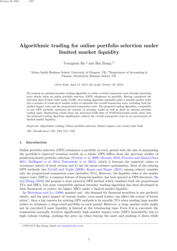
October 30, 2018AT52.2.Implementation shortfall algorithmA path-dependent or dynamic trading strategy by Lorenz (2008, Chapter 2–3), where the tradingpath is updated by real-time data, is superior in terms of generating a more efficient frontier to thepath-independent or static trading strategy by Almgren and Chriss (2001), where the trading pathis determined before trading starts. The superiority of the dynamic strategy comes from tradingfaster and reducing the risk of price volatility for the remaining time in the future if there was awindfall trading gain (i.e. lower trading cost) in the past.Two other trading strategies as in Almgren and Chriss (2001), Guéant et al. (2012) respectivelyare similar in terms of liquidating a certain quantity of a single-asset portfolio within a given timehorizon. However, they are different in terms of order types and optimisation methods. The formersends market orders by considering the trade-off between price risk and MICs, whereas the lattersends limit orders by considering both price risk and non-execution risk. Moreover, the Almgrenand Chriss’s strategy uses quadratic programming to construct an efficient frontier where thetrade-off between price risk and MICs is binding, whereas the Guéant et al.’s strategy applies theHamilton–Jacobi–Bellman equation to solve the stochastic control problem of optimal liquidation.2.3.Black box algorithmThe following types of black box algorithm are reviewed: Pairs tradingStatistical arbitrage strategies based on cointegrated pairs of assets; High-frequency tradingShort-term trading strategies using sophisticated mathematics and high-speed computers; Artificial intelligence tradingAlpha generation strategies using artificial intelligence techniques.2.3.1.Pairs trading. Avellaneda and Lee (2010) constructed a statistical arbitrage strategyof a market-neutral long–short portfolio. To be specific, they used pairs trading: long one dollar ina stock and short βj dollars in the j-th factor, where a multi-factor regression model decomposes astock return R into the sum of systematic components mj 1 βj Fj (m is the number of factors) andan idiosyncratic component R̃:mR βj Fj R̃.(1)j 1This method generates trading signals of buy, sell, or close of the long (short) position by using themean-reverting property of the long–short portfolio’s return.Similar to Avellaneda and Lee (2010), Caldeira and Moura (2013) also considered a market-neutralstrategy but used a different long–short portfolio. Avellaneda and Lee’s strategy constructed eithera pair of one stock and multiple exchange-traded funds or a pair of one stock and factors calculatedfrom the principal component analysis while Caldeira and Moura constructed only two stocksas a pair. Moreover, if these two stocks selected are cointegrated, then it is possible to form amean-reverting stationary process from a linear combination of stock A and B.2.3.2.High-frequency trading. A Markov chain model of the short-term dynamics of a LOBwas proposed by Cont et al. (2010). To be specific, the volume of limit orders (see Table 1) ismodelled as a Markov state, where a state transition occurs by a limit order, a market order,or a stop order. Furthermore, this model can be applied to high-frequency trading by making ashort-term prediction of the mid-price and making a round-trip transaction. It enters a long position4

October 30, 2018AT5when the probability of the mid-price increasing is high, and it exits the position either when aprofit is secured or when a loss of one tick is made.A high-frequency arbitrage opportunity through an empirical analysis of the LOB resiliency ofstocks traded on Shenzhen Stock Exchange was found (Xu et al. 2017). The analysis showed thatbuy (sell) market orders attract more buy (sell) limit orders especially i) when the bid-ask spread isone tick and ii) when the buy (sell) market order size is less than the best ask (bid) volume, whichis the volume of LOB at level 1 ( 1) (see Table 1).2.3.3.Artificial intelligence trading. Tan et al. (2011) explained how to detect stock cyclesfrom historical stock prices. Based on the mean reverting property of stock prices they provideda reinforcement learning framework to trade on the cycles. Specifically, long positions are heldafter detecting troughs of stock cycles, and short positions are held after detecting peaks of stockcycles. In addition, a dynamic asset switching strategy was proposed to detect buying opportunities(troughs) of all assets in a portfolio.Mousavi et al. (2014) proposed a multi-tree genetic programming model that i) extracts profitabletrading rule bases for a multi-asset portfolio from historical data (daily closing price and transactionvolume) and ii) updates the portfolio weights over time. Even though it generates a distinct decisionrule for each stock, the rules for multiple stocks evolve simultaneously, and the correlations amongmultiple stocks are taken into account. In addition, the proposed model includes the risks andtransaction costs to make the trading system more realistic.Bendtsen and Peña (2016) developed a single-asset trading algorithm with either a long or closedposition (i.e. no short selling) by using technical indicators such as moving average and relativestrength index. Its goal is to generate buy or sell signals for trading a stock by learning andpredicting the stock movement. A gated Bayesian network has been adopted to create a lower riskinvestment strategy compared with the buy-and-hold strategy. The network goes back and forthbetween the buy and sell phases and seeks opportunities to buy or sell shares.Krauss et al. (2017) generated daily trading signals from lagged returns of stocks. They conductednonparametric nonlinear regression between the lagged returns and one-day-ahead return. Inparticular, the following nonlinear regression methods were employed: deep neural networks,gradient-boosted trees, and random forests. After the regression, a daily portfolio of either goinglong for the stocks of higher expected returns or going short for lower expected return stocks hasbeen constructed from the combined signals of the three methods.3.NotationsThe following notations are used in this paper: A lower case italic letter x indicates a deterministic scalar value, while a capital italic letter Xindicates a random variable. A lower case italic bold letter x indicates a deterministic vector,while a capital italic bold letter X indicates a multivariate random variable (i.e. a randomvector). A capital upright bold letter X denotes a deterministic matrix or a random matrix. R {x R x 0} denotes positive real numbers.(1)(2) b n [bn bn(d) T. . . bn ] is a portfolio vector of d risky assets (there is no risk-free asset in the(j )portfolio) on the n-th day (see Figure 2), where n {1, 2, . . .}, bn 0 R (i.e. neither short(j )(j )selling nor buying stocks on margin is permitted), and dj 1 bn 1 (i.e. bn is the proportionof a portfolio invested in asset j {1, 2, . . . , d} at the n-th day). Hence, b n d 1 , whereT d 1 {[b(1) b(2) . . . b(d) ] Rd dj 1 b(j ) 1, b(j ) 0} is the standard (d 1)-simplex. b n,t d 1 is an intraday portfolio vector at time t after the end of the n-th day, wheret {0, 1, . . . , τ }, and τ is the number of intraday trades (see Figure 2; the portfolio rebalancing5

October 30, 2018AT5portfoliob2b n 1portfolio rebalancingb1from b n to b n 1 bnat the present momentb n 11st day(n 1)-th dayn-th day0mn 1 was givenat the end ofthe (n 1)-th day(past)mn is being givenat the end ofthe n-th day(present)timeMn 1 will be givenat the end ofthe (n 1)-th day(future)portfolio bnmn,0 is being givenat time 0(after orat market opening)after the end ofthe n-th dayb n,3b n,2b n,1b n,τb n 1 Mn,1 will be givenat time 1after the end ofthe n-th dayMn,2 will be givenat time 2after the end ofthe n-th day Mn,τ will be givenat time τ(before orat market closing)after the end ofthe n-th daytimeFigure 2. The timeline of intraday trading when the present moment is the end of n-th day. OPS rebalances aportfolio at the end of every trading day (a day ends at time 0, e.g. 9:30 a.m. or 10:00 a.m., not midnight, in thispaper), and an algorithmic trading strategy cushions the shock by portfolio rebalancing from b n to b n 1 .from b n,τ to b n 1 is not counted as an intraday trade).T b 1 [1/d 1/d . . . 1/d] is an initial portfolio vector.(j )(j ) A deterministic value mn (if n is a past or present day), or a random variable Mn (if n is afuture day) is the mid-price of asset j at the end of the n-th day.(j )(j ) A deterministic value mn,t (if n, t is in the past or at the present), or a random variable Mn,t(if n, t is in the future) is the mid-price of asset j at time t after the end of the n-th day.(j )(j )(j )(j )Technically, mn,0 mn and Mn,0 Mn . A deterministic value(j )xn (j )mn(j )Xn(j )Mn, or a random variable (j )(j )mn 1Mn 1the relative price of asset j for one day at the end of the n-th day.(1)(2) A deterministic vector x n [xn xn(1)(2)(j ) Mn (j )or Xn (j ) is mn 1 (d) T. . . xn ] Rd , or a multivariate random variable(d) TX n [Xn Xn . . . Xn ] Rd is the vector of the relative prices of all assets at the end ofthe n-th day (x n or X n is called a market vector in this paper).6

October 30, 2018AT5(j )(j )(j )Mn,t (j ) A deterministic value (j ) , or a random variable (j )or Xn,t (j )mn,t 1Mn,t 1 mn,t 1 is the intraday relative price of asset j between time t 1 and t after the end of the n-th day,defdefwhere mn, 1 mn 1,τ , and Mn, 1 Mn 1,τ .(j )xn,tmn,t(1)(j )Xn,tMn,t(d) T(2) A deterministic vector x n,t [xn,t xn,t . . . xn,t ] Rd , or a multivariate random variable(1)(2)(d) TX n,t [Xn,t Xn,t . . . Xn,t ] Rd is the vector of the intraday relative prices of all assets, attime t after the end of the n-th day (x n,t or X n,t is called an intraday market vector in thispaper).4.4.1.Market impact costs and transaction cost factorMarket impact costs (MICs) as a function of order size in a limit order bookMIC is incurred when rebalancing a portfolio, and it can be written as a function of order volumesand prices in LOBs. The average MIC as a function of order size q is defined as (Olsson 2005,Chapter 2.3)π (q, m, p1 , p2 , . . . , p 1 , p 2 , . . . , v1 , v2 , . . . , v 1 , v 2 , . . .)def p̄(q, m, p1 , p2 , . . . , p 1 , p 2 , . . . , v1 , v2 , . . . , v 1 , v 2 , . . .) m m(2),where m p 12 p1 is the midpoint between the best bid and the best ask price, called mid-price. Theaverage price per share for the order size q is defined asp̄(q, m, p1 , p2 , . . . , p 1 , p 2 , . . . , v1 , v2 , . . . , v 1 , v 2 , . . .) 1 1 pv p(q vi ) iik i k 1i k 1 , q p 1 , def m, p1 , k 1k 1 pi vi pk (q vi ) i 1i 1 , qif q v 1if v 1 q 0,if q 0if 0 q v1(3)if v1 qwhere positive (negative) q means buying (selling) stocks, pi and vi with positive (negative) i arethe quoted ask (bid) price and volume at level i, respectively (pi and vi correspond to the secondand third column of Table 1, respectively, where vi 0, v i 0, i {1, 2, . . .}), and the highest(lowest) trading level k when q v1 (q v 1 ) isx 1xi 1i 1k {x Z x 2, vi q vi } ,7(4a)

October 30, 2018AT5 1 1i xi x 1(k {x Z x 2, vi q vi }) ,(4b)i.e. k represents the level in the order book where the q-th share would be executed.4.2.Transaction cost factor with both proportional transaction costs and marketimpact costsThe net wealth at time t after the end of the n-th day is a deterministic value νn,t if n, t is in thepast or at the present; while it is a random variable Nn,t if n, t is in the future (the notations ofrandom variables are omitted in the subsequent expressions). The net wealth is defined asdefνn,t sn,t γn,t ,(5)where sn,t is the gross wealth at time t after the end of the n-th day, and γn,t is transaction cost(TC) at time t after the end of the n-th day. The gross wealth sn,t can be calculated from theprevious net wealth νn,t 1 :d(j ) (j )sn,t νn,t 1 bn,t xn,t νn,t 1 ⟨b n,t , x n,t ⟩,(6)j 1defwhere νn, 1 νn 1,τ , and ⟨ , ⟩ denotes the inner product. Transaction cost factor (TCF) at time tafter the end of the n-th day is defined as (Györfi and Vajda 2008)defwn,t νn,t,sn,t(7)where wn,t (0, 1] γn,t [0, sn,t ).Let us calculate wn,t when rebalancing from b n,t to b n,t 1 . Followed by (Ha and Zhang 2018,Section 5.2–5.3), the gross wealth sn,t , the sum of the net wealth νn,t , the MICs, the purchase TCs,and the sale TCs, is given byd(j )(j )(j )d(j )d(j ) (j )(j ) sn,t νn,t (p̄ (qn,t ) mn,t ) qn,t cp (p̄ (qn,t ) qn,t ) cs ( p̄ (qn,t ) qn,t ) ,j 1j 1(8)j 1where cp , cs [0, 1) denotes the rate of proportional TCs when purchasing and selling stocksrespectively and a max(0, a).def2(j )qn,t(j )(j )qn,t is an unknown order size of asset j:(j ) (j ) (j )bn,t 1 sn,t wn,t bn,t xn,t νn,t 1(j );(9)mn,tdef (j )and bn,τ 1 bn 1 . Equation (8) can be simplified, by the property of a a ( a) , asd(j )(j )(j )d(j )(j ) sn,t νn,t ((1 cs )p̄ (qn,t ) mn,t ) qn,t (cp cs ) (p̄ (qn,t ) qn,t ) ,j 12(10)j 1Some arguments of Equation (3), m, p1 , p2 , . . . , p 1 , p 2 , . . . , v1 , v2 , . . . , v 1 , v 2 , . . . of asset j, are omitted in Equation (8)and the subsequent expressions for notational simplicity8

October 30, 2018AT5and this can be rewritten, using Equation (7), as(j )wn,t 1 (j )(j )(j )(j ) dd j 1 ((1 cs )p̄ (qn,t ) mn,t ) qn,t (cp cs ) j 1 (p̄ (qn,t ) qn,t )sn,t,(11)defwhere w0,t 1, t {0, 1, . . . , τ } (i.e. there are no TCs between time 0 and τ on the0-th day). Equation (9) and (11) are solvable by using a root-finding algorithm, wherewn,t w (b n,t , b n,t 1 , x n,t , νn,t 1 ) is an unknown variable, cp and cs are omitted here for notationalsimplicity.5.Proposed method of optimal intraday tradingThis section explains:(i) how to calculate the expected value of the gross wealth of tomorrow in the case of nointraday trading (i.e. τ 0);(ii) how to obtain an optimal trading path when rebalancing a portfolio from b n to b n 1 , giventhe number of intraday trades τ 1 (see Figure 2);(iii) how to calculate the optimal number of intraday trades τ ;(iv) and how to consider real-time LOB data for optimal intraday trading.The following assumptions are made for the simplicity of the proposed method:Assumption 5.1 Asset prices follow the multi-dimensional Brownian motion with zero drift (forecasting expected returns is not performed in this paper); hence, the increments of asset prices are jointly normally distributed; and the increments of asset prices are mutually independent for different assets j j ′ ordifferent trading times t t′ .Assumption 5.2 LOB at time t′ {t 1, t 2, . . . , τ } is the same as LOB at time t on the sameday.5.1.No intraday trading (τ 0)Suppose that a filtered probability space (Ω, F , {Fn }n {1,2,.} , P) is given, where Fn denotes thenatural filtration of the process {X n }n {1,2,.} up to day n. If no intraday trading occurs, theconditional expected value of the gross wealth at the end of the (n 1)-th day, given the pastobservations x 1 , x 2 , . . . , x n , and using Equation (6) and (7), is given byE[Sn 1 Fn ] E[Nn ⟨b n 1 , X n 1 ⟩ Fn ] E[Sn Wn ⟨b n 1 , X n 1 ⟩ Fn ] E[Sn Wn Fn ]E[⟨b n 1 , X n 1 ⟩ Fn ](12) sn wn E[⟨b n 1 , X n 1 ⟩],where Nn is stochastic net wealth at the end of the n-th day, Sn s0 ni 1 ⟨b i , X i ⟩ is stochastic gross wealth at the end of the n-th day with an initial wealths0 ,9

October 30, 2018AT5 Wn w(b n , b n 1 , X n , Nn 1 ) is stochastic TCF at the end of the n-th day (Sn Wn and⟨b n 1 , X n 1 ⟩ are mutually independent by Assumption 5.1 that X n and X n 1 are mutually independent), sn s0 ni 1 ⟨b i , x i ⟩ is deterministic gross wealth at the end of the n-th day, wn w(b n , b n 1 , x n , νn 1 ) is deterministic TCF at the end of the n-th day (Sn Wn is convertedto sn wn by the conditional expectation given Fn ), and the market vector X n 1 is jointly normally distributed with the mean vector of all 1’s[1 1 . . . 1]T .By Assumption 5.1, Equation (12) can be further simplified, and the price change M n 1 m nfollows the multi-dimensional Brownian motion with zero drift:(M n 1 m n ) N (0 , Σn ),(1)(13)(d ) T(2)where M n 1 [Mn 1 Mn 1 . . . Mn 1 ] is the random mid-price vector at the end of the (n 1)-th(1)(2)(d) Tday, m n [mn mn . . . mn ] is the deterministic mid-price vector at the end of the n-th day,0 denotes the all-zero vector, and Σn is the covariance matrix of price changes between the end ofthe n-th day and the end of the (n 1)-th day. Hence, M n 1 is jointly normally distributed asM n 1 N (m n , Σn ).(14)X n 1 D 1 M n 1 ,(15)Also, as X n 1 can be calculated aswhere D diag(m n ), it is jointly normally distributed asX n 1 N (1 , D 1 Σn D 1 ) .(16)Consequently, E[Sn 1 Fn ] in Equation (12) can be simplified asE[Sn 1 Fn ] sn wn E[⟨b n 1 , X n 1 ⟩](1)(1)(2)(2)(d)(d) sn wn E [bn 1 Xn 1 bn 1 Xn 1 bn 1 Xn 1 ](1)(1)(2)(2)(d )(d ) sn wn (bn 1 E [Xn 1 ] bn 1 E [Xn 1 ] bn 1 E [Xn 1 ])d(17)(j ) sn wn bn 1j 1 sn wn .5.2.Single intraday trade (τ 1)If there is noly one intraday trading per trading day, then the conditional expected value of thegross wealth at the end of the (n 1)-th day, given the past observations x 1 , x 2 , . . . , x n , and usingEquation (6), (7), and (12), is given byE[Sn 1 Fn ] sn wn E[⟨b n,1 , X n,1 ⟩Wn,1 ⟨b n 1 , X n 1,0 ⟩],where10(18)

October 30, 2018AT5 wn w(b n , b n,1 , x n,0 , νn 1,1 ) (wn is TCF at the end of the n-th day when rebalancing aportfolio from b n to b n,1 ),m(n1)m(n2)(1)mn 1,1 m(n2 )1,1(j )though mn,0 is x n,0 [even X n,1 [(2)(1)Mn,1Mn,1m(n1)m(n2).m(nd)m(nd )1,1T] (x n,0 is not equivalent to x n [(j )X n 1 [X n 1,0 [(d)Mn,1m(nd)Mn(1 )1 Mn(2 )1(1)mn(2)mnMn,1.m(nd)m(nd )1T]T] ,Mn(1 )1 Mn(2 )1(1).equivalent to mn ), Wn,1 w(b n,1 , b n 1 , X n,1 , sn wn ), and(2)m(n1) mn(1)(2)mn 1 mn 1(2)Mn,1Mn(d )1(d)mn.Mn(d )1(d)Mn,1]T(X n 1,0Tisnot(j )equivalentto(j )] even though Mn 1,0 is equivalent to Mn 1 ).Of course, the MIC function in Equation (2) at time 1 after the end of the n-th day to calculateWn,1 is stochastic as LOBs are continuously updated by other investors between time 0 and 1.(j )(j )However, the random variables Pi , Vi , i, j in LOBs at time 1 are omitted in Equation (18)(j )(j )for the simple expression, where Pi (Vi ) is a random variable of the quoted price (volume) ofasset j at level i in LOBs. This corresponds to Assumption 5.2.By Assumption 5.1 that the two random vectors X n,1 , X n 1,0 are mutually independent, Equation (18) can be rewritten again asE[Sn 1 Fn ] sn wn E[⟨b n,1 , X n,1 ⟩Wn,1 ]E[⟨b n 1 , X n 1,0 ⟩],(19)but ⟨b n,1 , X n,1 ⟩ and Wn,1 are mutually dependent as Wn,1 is a function of X n,1 . Finally, by theproperty of E[⟨b n 1 , X n 1,0 ⟩] 1, as proved in Equation (17), E[Sn 1 Fn ] in Equation (18) can besimplified asE[Sn 1 Fn ] sn wn E[⟨b n,1 , X n,1 ⟩Wn,1 ].(20)Our goal is to find the optimal portfolio vector b n,1 that maximises E[Sn 1 Fn ], and this is astochastic programming problem defined as follows:b n,1 arg max E[Sn 1 Fn ]b n,1 d 1 arg max sn wn E[⟨b n,1 , X n,1 ⟩Wn,1 ]b n,1 d 1 arg max wn E[⟨b n,1 , X n,1 ⟩Wn,1 ](21)b n,1 d 1 arg max wn b n,1 d 1x n,1 Rd ⟨b n,1 , x n,1 ⟩wn,1 f (x n,1 )dx n,1 ,where wn,1 w(b n,1 , b n 1 , x n,1 , sn wn ), f (x n,1 ) is the probability density function (PDF)of the multivariate normal distribution X n,1 N (1 , D 1 Σn,1 D 1 ), and D diag(m n )(arg maxb n,1 d 1 sn wn E[⟨b n,1 , X n,1 ⟩Wn,1 ] is equivalent to arg maxb n,1 d 1 wn E[⟨b n,1 , X n,1 ⟩Wn,1 ]as the gross wealth at the end of the n-th day sn s0 ni 1 ⟨b i , x i ⟩ is independent of b n,1 ). As aresult, not only forecasting the covariance matrix of price changes between time 0 and 1 after theend of the n-th day Σn,1 (i.e. multivariate intraday volatility), but also calculating the Monte Carlonumerical integration (a closed-form solution of E[Sn 1 Fn ] does not exist as that of wn,1 does not)is required to obtain b n,1 .Therefore, to avoid both the intraday forecasting of volatility and the heavy computation ofintegration (ultimately, to make the stochastic programming problem in Equation (21) simpler), the11

AT500.80.2b (3)0.6b(1)(2)0.40.40.60.20.8b(2)b0.40.20.60.40.6b n,1 b n,1 (cs 0%) b n,1 (cs 10%) b n,1 (cs 20%)b n 10.80.20.60.400b n,1 b n,1 (cs 0%) b n,1 (cs 10%) b n,1 (cs 20%)b n 1b (3)October 30, 201800.80

High-frequency trading Short-term trading strategies using sophisticated mathematics and high-speed computers; Artificial intelligence trading Alpha generation strategies using artificial intelligence techniques. 2.3.1. Pairs trading. Avellaneda a