WIXLIB

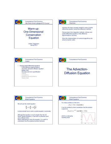
Computational Fluid Dynamicshttp://www.nd.edu/ rvationEquation!Computational Fluid DynamicsObjectives:!Introduce the basic concepts needed to solve a partialdifferential equation using finite difference methods. !!Discuss basic time integration methods, ordinary andpartial differential equations, finite differenceapproximations, accuracy. !!Show the implementation of numerical algorithms intoactual computer codes.!Grétar Tryggvason!Spring 2013!Computational Fluid DynamicsOutline! Solving partial differential equations!! !Finite difference approximations!! !The linear advection-diffusion equation!! !Matlab code!! !Accuracy and error quantification!! !Stability!! !Consistency!! !Multidimensional problems!! !Steady state!Computational Fluid DynamicsModel Equations!We will use the model equation:! f f 2 f U D 2 t x xComputational Fluid DynamicsThe AdvectionDiffusion Equation!Computational Fluid DynamicsModel Equations!For initial conditions of the form:!f (x, t 0) Asin(2πkx)It can be verified by direct substitution that the solutionis given by:!f (x, t) e Dk t sin(2πk(x Ut))2to demonstrate how to solve a partial equation numerically.!Although this equation is much simpler than the fullNavier Stokes equations, it has both an advection termand a diffusion term. !Before attempting to solve the equation, it is useful tounderstand how the analytical solution behaves.!which is a decayingtraveling wave!

Computational Fluid DynamicsConservation equations!Computational Fluid DynamicsConservation equations!Most physical laws are based on CONSERVATIONprinciples: In the absence of explicit sources or sinks, fis neither created nor destroyed.!!Consider a simple one dimensional pipe of uniformdiameter with a given velocity !f (t)To predict the evolution of f everywhere in the pipe,we assume that f is conserved. Thus, for any sectionof the pipe:!Amount of fin a controlvolumeafter agiven timeinterval Δt!U (x)xGiven f at the inlet as a function of time (as well aseverywhere at time zero), how do we predict the f(t,x)? ! Amount of f inthe controlvolume at thebeginning ofthe timeinterval Δt! Amount off thatflows intothe controlvolumeduring Δt!-Amount off that flowsout of thecontrolvolumeduring Δt!U (x)f (t)xΔxComputational Fluid DynamicsConservation equations!How much does the total amount of f inthe Control Volume change during a shorttime Δt? Restating the conservation lawfrom the last slide, we have!Computational Fluid DynamicsConservation equations!We can also state the conservation principlein differential form. From last slide!Total f (t Δt) –total f (t) Total inflow of f - Total outflow of fApproximate:!fTotal xf dx f av ΔxDenote the flow rate of f into the control volume by F then:!()() f av t Δt f av t Δx Δt Fin Fout Computational Fluid DynamicsConservation equations!()() f av t Δt f av t Δx Δt Fin Fout ΔxΔxDivide by ΔtΔx!!()() f av t Δt f av t Fout Fin ΔtΔxor:!Δf avΔF ΔtΔxTaking thelimit, we get:! f F 0 t xF: Flux of f!Computational Fluid DynamicsThe general form of the one-dimensionalconservation equation is:! f F 0 t xTaking the flux to be the sum of advective anddiffusive fluxes:!F Uf F f xGives the advection diffusion equation! f f 2 f U D 2 t x xFinite DifferenceApproximations ofthe Derivatives!

Computational Fluid DynamicsFinite Difference Approximations!Computational Fluid DynamicsFinite Difference Approximations!Derive a numerical approximation to the governingequation, replacing a relation between the derivatives bya relation between the discrete nodal values.!f (t 2Δt)ΔtΔtThe!Time Derivative!f (t Δt)f(t,x-h) f(t,x) f(t,x h) !hf (t)hComputational Fluid DynamicsFinite Difference Approximations!Computational Fluid DynamicsFinite Difference Approximations!Time derivative!The Time Derivative is found using a FORWARDEULER method. The approximation can be found byusing a Taylor series!f(t Δt,x)Δtf(t,x)!hhComputational Fluid DynamicsFinite Difference Approximations!The Spatial!First Derivative!f (t Δt) f (t) f (t) 2 f (t) Δt 2Δt t t 2 2Solving this equation for the time derivative gives:! f (t) f (t Δt) f (t) 2 f (t) Δt tΔt t 2 2Computational Fluid DynamicsFinite Difference Approximations!When using FINITE DIFFERENCE approximations,the values of f are stored at discrete points.!f(x-h) f(x) f(x h) !hhThe derivatives of the function are approximatedusing a Taylor series!

Computational Fluid DynamicsFinite Difference Approximations!Start by expressing the value of f(x h) and f(x-h) in terms of f(x) f (x) 2 f (x) h 2 3 f (x) h 3 4 f (x) h 4f (x h) f (x) h x x 2 2 x 3 6 x 4 24f (x h) f (x) f (x) 2 f (x) h 2 3 f (x) h 3 4 f (x) h 4h x x 2 2 x 3 6 x 4 24Subtracting the second equation from the first:!f (x h) f (x h) 2 f (x) 3 f (x) h 3h 2 x x 3 6Computational Fluid DynamicsFinite Difference Approximations!The result is:!f (x h) f (x h) 2 f (x) 3 f (x) h 3h 2 x x 3 6Rearranging this equation to isolate the first derivative:! f (x) f (x h) f (x h) 3 f (x) h 2 x2h x 3 6Computational Fluid DynamicsFinite Difference Approximations!Computational Fluid DynamicsFinite Difference Approximations!Start by expressing the value of f(x h) and f(x-h) in terms of f(x)The Spatial!Second Derivative!f (x h) f (x) f (x) 2 f (x) h 2 3 f (x) h 3 4 f (x) h 4h x x 2 2 x 3 6 x 4 24f (x h) f (x) f (x) 2 f (x) h 2 3 f (x) h 3 4 f (x) h 4h x x 2 2 x 3 6 x 4 24Adding the second equation to the first:!f (x h) f (x h) 2 f (x) 2Computational Fluid DynamicsFinite Difference Approximations! f 2 (x) h 2 4 f (x) h 4 2 2 x2 x 4 24Computational Fluid DynamicsFinite Difference Approximations!The result is:!f (x h) f (x h) 2 f (x) 2 f 2 (x) h 2 4 f (x) h 4 2 2 x2 x 4 24Rearranging this equation to isolate the second derivative:! 2 f (x) f (x h) 2 f (x) f (x h) 4 f (x) h 2 x 2h2 x 4 12Solving the partialdifferential equation!

Computational Fluid DynamicsFinite Difference Approximations!Computational Fluid DynamicsFinite Difference Approximations!A numerical approximation to!Use the notation! f n f (t)For space and time we will use:! f f 2 f U D 2 t x xnf j f (t, x j )f jn 1f jn 1Is found by replacing the derivatives by the followingapproximations!f jn 1 f (t Δt, x j )f jn 1 f (t, x j h)f jn f jn 1hf jn 1 f (t, x j h)nnn 2 f f f U D 2 t j x j x jΔthf jn 1f jn 1f jn f jn 1hComputational Fluid DynamicsFinite Difference Approximations!hComputational Fluid DynamicsFinite Difference Approximations!Substituting these approximations into:!Using the shorthand !notation!gives!f fj f j O(Δt) t jΔtnf jn f (t, x j )f jn 1 f (t Δt, x j )n 1 f f 2 f U D 2 t x xngives!f f j 1 f j 1 O(h2 ) x j2hnf jn 1 f (t, x j h)f jn 1 f (t, x j h)nnf jn 1 fjnf jn 1 fjn 1fjn 1 2 f jn f jn 1 U D O(Δt, h 2 )Δt2hh2n 2 f f jn 1 2 f jn f jn 12 O(h )2 x jh2Solving for the new value and dropping the error terms yields!fjComputational Fluid DynamicsFinite Difference Approximations!n 1 fj nUΔt nDΔt nnnn( f f j 1) 2 ( f j 1 2 f j f j 1)2h j 1hComputational Fluid DynamicsThus, given f at one time (or time level), f at thenext time level is given by:!f jn 1 f jn ΔtUΔt nDΔt( f j 1 f jn 1) 2 ( f jn 1 2 f jn f jn 1)2hhThe value of every point at level n 1 is givenexplicitly in terms of the values at the level n!f jn 1f jn 1f jn f jn 1hhΔtExample!

Computational Fluid DynamicsA short MATLAB program!The evolution of a sine wave is followed as itis advected and diffused. Two waves of theinfinite wave train are simulated in a domain oflength 2. To model the infinite train, periodicboundary conditions are used. Compare thenumerical results with the exact solution.!Computational Fluid DynamicsEX2!% one-dimensional advection-diffusion by the FTCS scheme!n 21; nstep 100; length 2.0; h length/(n-1); dt 0.05; D 0.05;!f zeros(n,1); y zeros(n,1); ex zeros(n,1); time 0.0;!for i 1:n, f(i) 0.5*sin(2*pi*h*(i-1)); end;% initial conditions!for m 1:nstep, m, time!for i 1:n, ex(i) ); end;% exact solution !hold off; plot(f,'linewidt',2); axis([1 n -2.0, 2.0]); % plot solution!hold on; plot(ex,'r','linewidt',2);pause;% plot exact solution!y f;% store the solution!for i 2:n-1,!f(i) y(i)-0.5*(dt/h)*(y(i 1)-y(i-1)) .!! D*(dt/h 2)*(y(i 1)-2*y(i) y(i-1)); % advect by centered differences!end;!f(n) y(n)-0.5*(dt/h)*(y(2)-y(n-1)) .!! D*(dt/h 2)*(y(2)-2*y(n) y(n-1));% do endpoints for!f(1) f(n);% periodic boundaries!time time dt;!end;!Computational Fluid DynamicsEvolutionfor!U 1;D 0.05;k 1N 21Δt 0.05Computational Fluid DynamicsAccuracy!Movie: adv1!Exact!Numerical!Computational Fluid DynamicsIt is clear that although the numerical solution isqualitatively similar to the analytical solution, thereare significant quantitative differences.!!The derivation of the numerical approximations forthe derivatives showed that the error depends onthe size of h and Δt. !!First we test for different Δt. !!Number of time steps T/ΔtComputational Fluid DynamicsAccuracy!Evolutionfor!U 1;D 0.05;k 1N 21Δt 0.05m 11; time 14161820

Computational Fluid DynamicsAccuracy!Computational Fluid DynamicsAccuracy!m 21; time 0.50!Repeat witha smallertime-step!Δt 0.025N 21m 41; time 0.50!Repeat witha smallertime-step!Δt 0.0125N nal Fluid DynamicsHow accurate solution canwe obtain?!!Take !Δt 0.0005 !and !N 200!-22468101214161820Computational Fluid DynamicsAccuracy!Very fine spatialresolution and asmall time step!m 1001; time 0.50!2U 1;D 0.05;k 1N 200Δt nal Fluid DynamicsQuantifying the Error!Order of Accuracy!-220406080100120140Computational Fluid DynamicsAccuracy!Examine the spatial accuracy by taking avery small time step, Δt 0.0005 and varythe number of grid points, N, used toresolve the spatial direction. !!The grid size is h L/N where L 1 for ourcase!160180200

Computational Fluid DynamicsAccuracy!Exact!time 0.50!Numerical!E hN ( fj 1N 11; E 0.1633!N 21; E 0.0403!N 41; E 0.0096!N 61; E 0.0041!N 81; E 0.0022!N 101; E 0.0015!N 121; E 0.0011!N 161; E 9.2600e-04! fexact )2jComputational Fluid DynamicsAccuracy!Accuracy. Effect of!spatial resolution!dt 0.0005!N 11 to N 161!time 0.50!10010-1-2E1010-310-4 0101011021021/ hComputational Fluid DynamicsAccuracy!Computational Fluid DynamicsAccuracy!time 0.50!If the error is of second order:! 2 1E Ch 2 C h Accuracy. Effect of!spatial resolution!10-1Taking the log:!-2E10 1 2 1ln E ln C lnC 2ln h h On a log-log plot, the E versus (1/h) curveshould therefore have a slope -2!Computational Fluid DynamicsAccuracy!Why is does the error deviate from the line for thehighest values of N?!Error!Truncation!Total!Roundoff!Number of Steps, N 1/h!1002!1!10-3dt 0.0005!!N 11 to N 161!10-4 0101011/ hComputational Fluid DynamicsSummary!Finite difference approximations by Taylorexpansion!!Approximating a partial differentialequation!!Showed, by numerical experiments, thataccuracy increases as the resolution isincreased!!Showed that the error behaves in a waythat should be predictable!

Navier Stokes equations, it has both an advection term and a diffusion term. ! Before attempting to solve the equation, it is useful to understand how the analytical solution behaves.! to demonstrate how to solve a partial equation numerically.! Model Equations! Computational Fluid Dynamics! For initial conditions of the form:! f(x,t 0) Asin(2πkx) f(x,t) e Dk2t sin(2πk(x Ut)) It can be .