Transcription
CHAPTER1Introduction toRadar Systemsand Signal Processing1.1History and Applications of RadarThe word “radar” was originally an acronym, RADAR, for “radio detection and ranging.”Today, the technology is so common that the word has become a standard English noun.Many people have direct personal experience with radar in such applications as measuringfastball speeds or, often to their regret, traffic control.The history of radar extends to the early days of modern electromagnetic theory (Swords,1986; Skolnik, 2001). In 1886, Hertz demonstrated reflection of radio waves, and in 1900 Tesladescribed a concept for electromagnetic detection and velocity measurement in an interview.In 1903 and 1904, the German engineer Hülsmeyer experimented with ship detection byradio wave reflection, an idea advocated again by Marconi in 1922. In that same year, Taylorand Young of the U.S. Naval Research Laboratory (NRL) demonstrated ship detection byradar and in 1930 Hyland, also of NRL, first detected aircraft (albeit accidentally) by radar,setting off a more substantial investigation that led to a U.S. patent for what would now becalled a continuous wave (CW) radar in 1934.The development of radar accelerated and spread in the middle and late 1930s, withlargely independent developments in the United States, Britain, France, Germany, Russia,Italy, and Japan. In the United States, R. M. Page of NRL began an effort to develop pulsedradar in 1934, with the first successful demonstrations in 1936. The year 1936 also saw theU.S. Army Signal Corps begin active radar work, leading in 1938 to its first operational system, the SCR-268 antiaircraft fire control system, and in 1939 to the SCR-270 early warningsystem, the detections of which were tragically ignored at Pearl Harbor. British development, spurred by the threat of war, began in earnest with work by Watson-Watt in 1935. TheBritish demonstrated pulsed radar that year, and by 1938 established the famous ChainHome surveillance radar network that remained active until the end of World War II. Theyalso built the first airborne interceptor radar in 1939. In 1940, the United States and Britainbegan to exchange information on radar development. Up to this time, most radar work wasconducted at high frequency (HF) and very high frequency (VHF) wavelengths; but with theBritish disclosure of the critical cavity magnetron microwave power tube and the UnitedStates formation of the Radiation Laboratory at the Massachusetts Institute of Technology,the groundwork was laid for the successful development of radar at the microwave frequencies that have predominated ever since.101 Richards ch01 p001-040.indd 122/11/13 4:50 PM
2Chapter OneEach of the other countries mentioned also carried out CW radar experiments, and eachfielded operational radars at some time during the course of World War II. Efforts in Franceand Russia were interrupted by German occupation. On the other hand, Japanese effortswere aided by the capture of U.S. radars in the Philippines and by the disclosure of Germantechnology. The Germans themselves deployed a variety of ground-based, shipboard, andairborne systems. By the end of the war, the value of radar and the advantages of microwavefrequencies and pulsed waveforms were widely recognized.Early radar development was driven by military necessity, and the military is still amajor user and developer of radar technology. Military applications include surveillance,navigation, and weapons guidance for ground, sea, air, and space vehicles. Militaryradars span the range from huge ballistic missile defense systems to fist-sized tacticalmissile seekers.Radar now enjoys an increasing range of applications. One of the most common is thepolice traffic radar used for enforcing speed limits (and measuring the speed of baseballsand tennis serves). Another is the “color weather radar” familiar to every viewer of localtelevision news. The latter is one type of meteorological radar; more sophisticated systemsare used for large-scale weather monitoring and prediction and atmospheric research.Another radar application that affects many people is found in the air traffic control systemsused to guide commercial aircraft both en route and in the vicinity of airports. Aviation alsouses radar for determining altitude and avoiding severe weather, and may soon use it forimaging runway approaches in poor weather. Radar is commonly used for collision avoidance and buoy detection by ships, and is now beginning to serve the same role for the automobile and trucking industries. Finally, spaceborne (both satellite and space shuttle) andairborne radar is an important tool in mapping earth topology and environmental characteristics such as water and ice conditions, forestry conditions, land usage, and pollution. Whilethis sketch of radar applications is far from exhaustive, it does indicate the breadth of applications of this remarkable technology.This text tries to present a thorough, straightforward, and consistent description of thesignal processing aspects of radar technology, focusing primarily on the more fundamentalfunctions common to most radar systems. Pulsed radars are emphasized over CW radars,though many of the ideas are applicable to both. Similarly, monostatic radars, where thetransmitter and receiver antennas are collocated (and in fact are usually the same antenna),are emphasized over bistatic radars, where they are significantly separated, though againmany of the results apply to both. The reason for this focus is that the majority of radar systems are monostatic, pulsed designs. Finally, the subject is approached from a digital signalprocessing (DSP) viewpoint as much as practicable, both because most new radar designsrely heavily on digital processing and because this approach can unify concepts and resultsoften treated separately.1.2Basic Radar FunctionsMost uses of radar can be classified as detection, tracking, or imaging. This text addresses allthree, as well as the techniques of signal acquisition and interference reduction necessary toperform these tasks.The most fundamental problem in radar is detection of an object or physical phenomenon. This requires determining whether the receiver output at a given time represents theecho from a reflecting object or only noise. Detection decisions are usually made by comparing the amplitude A(t) of the receiver output (where t represents time) to a threshold T(t),which may be set a priori in the radar design or may be computed adaptively from the radardata; in Chap. 6 it will be seen why this detection technique is appropriate. The time requiredfor a pulse to propagate a distance R and return, thus traveling a total distance 2R, is just01 Richards ch01 p001-040.indd 222/11/13 4:50 PM
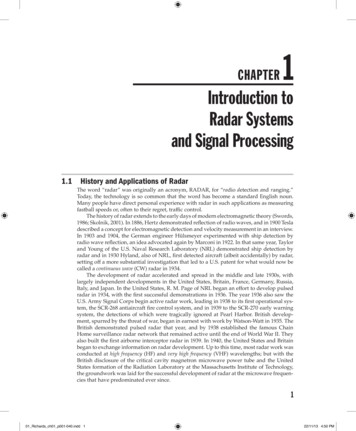
Introduction to Radar Systems and Signal Processing3FIGURE 1.1 Spherical coordinate system for radar measurements.2R/c; thus, if A(t) T(t) at some time delay t0 after a pulse is transmitted, it is assumed thata target is present at rangeR ct02(1.1)where c is the speed of light.1Once an object has been detected, it may be desirable to track its location or velocity. Amonostatic radar naturally measures position in a spherical coordinate system with its origin at the radar antenna’s phase center, as shown in Fig. 1.1. In this coordinate system, theantenna look direction, sometimes called the boresight direction, is along the x axis. Theangle q is called azimuth angle, while f is called elevation angle. Range R to the object followsdirectly from the elapsed time from transmission to detection as just described. Elevationand azimuth angle f and q are determined from the antenna orientation, since the targetmust normally be in the antenna main beam to be detected. Velocity is estimated by measuring the Doppler shift of the target echoes. Doppler shift provides only the radial velocitycomponent, but a series of measurements of position and radial velocity can be used to infertarget dynamics in all three dimensions.Because most people are familiar with the idea of following the movement of a “blip” onthe radar screen, detection and tracking are the functions most commonly associated withradar. Increasingly, however, radars are being used to generate two-dimensional images of anarea. Such images can be analyzed for intelligence and surveillance purposes, for topologymapping, or for analysis of earth resources issues such as mapping, land use, ice cover analysis, deforestation monitoring, and so forth. They can also be used for “terrain following” navigation by correlating measured imagery with stored maps. While radar images have notachieved the resolution of optical images, the very low attenuation of electromagnetic wavesat microwave frequencies gives radar the important advantage of “seeing” through clouds,fog, and precipitation very well. Consequently, imaging radars generate useful imagery whenoptical instruments cannot be used at all.1c 2.99792458 108 m/s in a vacuum. A value of c 3 108 m/s is normally used except where veryhigh accuracy is required.01 Richards ch01 p001-040.indd 322/11/13 4:50 PM
4Chapter OneThe quality of a radar system is quantified with a variety of figures of merit, dependingon the function being considered. In analyzing detection performance, the fundamentalparameters are the probability of detection PD and the probability of false alarm PFA. If other system parameters are fixed, increasing PD always requires accepting a higher PFA as well. Theachievable combinations are determined by the signal and interference statistics, especiallythe signal-to-interference ratio (SIR). When multiple targets are present in the radar field ofview, additional considerations of resolution and sidelobes arise in evaluating detection performance. For example, if two targets cannot be resolved by a radar, they will be registeredas a single object. If sidelobes are high, the echo from one strongly reflecting target maymask the echo from a nearby but weaker target, so that again only one target is registeredwhen two are present. Resolution and sidelobes in range are determined by the radar waveform, while those in angle are determined by the antenna pattern.In radar tracking, the basic figure of merit is accuracy of range, angle, and velocity estimation. While resolution presents a crude limit on accuracy, with appropriate signal processing the achievable accuracy is ultimately limited in each case by the SIR.In imaging, the principal figures of merit are spatial resolution and dynamic range. Spatial resolution determines what size objects can be identified in the final image, and thereforeto what uses the image can be put. For example, a radar map with 1 km by 1 km resolutionwould be useful for land use studies, but useless for military surveillance of airfields or missile sites. Dynamic range determines image contrast, which also contributes to the amountof information that can be extracted from an image.The purpose of signal processing in radar is to improve these figures of merit. SIR can beimproved by pulse integration. Resolution and SIR can be jointly improved by pulse compression and other waveform design techniques, such as frequency agility. Accuracy benefitsfrom increased SIR and interpolation methods. Sidelobe behavior can be improved with thesame windowing techniques used in virtually every application of signal processing. Eachof these topics are discussed in the chapters that follow.Radar signal processing draws on many of the same techniques and concepts used inother signal processing areas, from such closely related fields as communications and sonar tovery different applications such as speech and image processing. Linear filtering and statisticaldetection theory are central to radar’s most fundamental task of target detection. Fourier transforms, implemented using fast Fourier transform (FFT) techniques, are ubiquitous, being usedfor everything from fast convolution implementations of matched filters, to Doppler spectrumestimation, to radar imaging. Modern model-based spectral estimation and adaptive filteringtechniques are used for beamforming and jammer cancellation. Pattern recognition techniquesare used for target/clutter discrimination and target identification.At the same time, radar signal processing has several unique qualities that differentiate itfrom most other signal processing fields. Most modern radars are coherent, meaning that thereceived signal, once demodulated to baseband, is complex-valued rather than real-valued.Radar signals have very high dynamic ranges of several tens of decibels, in some extreme casesapproaching 100 dB. Thus, gain control schemes are common, and sidelobe control is oftencritical to avoid having weak signals masked by stronger ones. SIR ratios are often relativelylow. For example, the SIR at the point of detection may be only 10 to 20 dB, while the SIR for asingle received pulse prior to signal processing is frequently less than 0 dB.Especially important is the fact that, compared to most other DSP applications, radarsignal bandwidths are large. Instantaneous bandwidths for an individual pulse are frequently on the order of a few megahertz, and in some fine-resolution2 radars may reach2Systems exhibiting good or poor resolution are commonly referred to as high- or low-resolutionsystems, respectively. Since better resolution means a smaller numerical value, in this text the terms“fine” and “coarse” are used instead.01 Richards ch01 p001-040.indd 422/11/13 4:50 PM
Introduction to Radar Systems and Signal erLocalOscillatorDisplayIF iseRFAmplifierFIGURE 1.2 Block diagram of a pulsed monostatic radar.several hundred megahertz and even as high as 1 GHz. This fact has several implications fordigital signal processing. For example, very fast analog-to-digital (A/D) converters arerequired. The difficulty of designing good converters at multi-megahertz sample rates hashistorically slowed the introduction of digital techniques into radar signal processing. Evennow, when digital techniques are common in new designs, radar word lengths in highbandwidth systems are usually a relatively short 8 to 12 bits, rather than the 16 bits commonin many other areas. The high data rates have also historically meant that it has often beennecessary to design custom hardware for the digital processor in order to obtain adequatethroughput, that is, to “keep up with” the onslaught of data. This same problem of providing adequate throughput has resulted in radar signal processing algorithms being relativelysimple compared to, say, sonar processing techniques. Only in the late 1990s has Moore’sLaw3 provided enough computing power to host radar algorithms for a wide range of systems on commercial hardware. Equally important, this same technological progress hasallowed the application of new, more complex algorithms to radar signals, enabling majorimprovements in detection, tracking, and imaging capability.1.3Elements of a Pulsed RadarFigure 1.2 is one possible block diagram of a simple pulsed monostatic radar. The waveformgenerator output is the desired pulse waveform. The transmitter modulates this waveformto the desired radio frequency (RF) and amplifies it to a useful power level. The transmitteroutput is routed to the antenna through a duplexer, also called a circulator or T/R switch (fortransmit/receive). The returning echoes are routed, again by the duplexer, into the radarreceiver. The receiver is usually a superheterodyne design, and often the first stage is alow-noise RF amplifier. This is followed by one or more stages of modulation of the received3Gordon Moore’s famous 1965 prediction was that the number of transistors on an integrated circuitwould double every 18 to 24 months. This prediction has held remarkably true for nearly 40 years,enabling the computing and networking revolutions that began in earnest in the 1980s.01 Richards ch01 p001-040.indd 522/11/13 4:50 PM
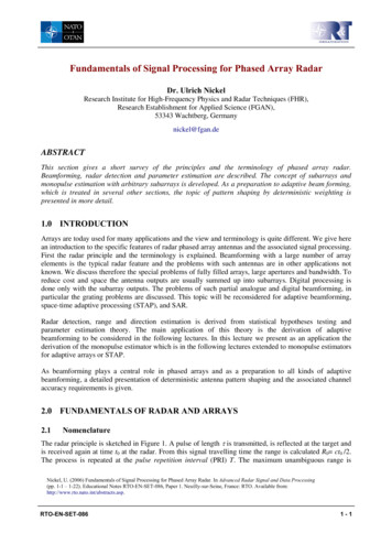
6Chapter Onesignal to successively lower intermediate frequencies (IFs) and ultimately to baseband, wherethe signal is not modulated onto any carrier frequency. Each modulation is carried out witha mixer and a local oscillator (LO). The baseband signal is next sent to the signal processor,which performs some or all of a variety of functions such as pulse compression, matchedfiltering, Doppler filtering, integration, and motion compensation. The output of the signalprocessor takes various forms, depending on the radar purpose. A tracking radar wouldoutput a stream of detections with measured range and angle coordinates, while an imagingradar would output a two- or three-dimensional image. The processor output is sent to thesystem display, the data processor, or both as appropriate.The configuration of Fig. 1.2 is not unique. For example, many systems perform some of thesignal processing functions at IF rather than baseband; matched filtering, pulse compression,and some forms of Doppler filtering are very common examples. The list of signal processingfunctions is redundant as well. For example, pulse compression and Doppler filtering can bothbe considered part of the matched filtering process. Another characteristic which differs amongradars is at what point in the system the analog signal is digitized. Older systems are, of course,all analog, and many currently operational systems do not digitize the signal until it is convertedto baseband. Thus, any signal processing performed at IF must be done with analog techniques.Increasingly, new designs digitize the signal at an IF stage, thus moving the A/D converter closerto the radar front end and enabling digital processing at IF. Finally, the distinction between signalprocessing and data processing is sometimes unclear or artificial.In the next few subsections, the major characteristics of these principal radar subsystemsare briefly discussed.1.3.1 Transmitter and Waveform GeneratorThe transmitter and waveform generator play a major role in determining the sensitivityand range resolution of radar. Radar systems have been operated at frequencies as low as2 MHz and as high as 220 GHz (Skolnik, 2001); laser radars operate at frequencies on theorder of 1012 to 1015 Hz, corresponding to wavelengths on the order of 0.3 to 30 µm (Jelalian,1992). However, most radars operate in the microwave frequency region of about 200 MHzto about 95 GHz, with corresponding wavelengths of 0.67 m to 3.16 mm. Table 1.1 summarizes the letter nomenclature used for the common nominal radar bands (IEEE, 1976). Themillimeter wave band is sometimes further decomposed into approximate subbands of 36 to46 GHz (Q band), 46 to 56 GHz (V band), and 56 to 100 GHz (W band) (Richards et al., 2010).Within the HF to Ka bands, specific frequencies are allocated by international agreement toradar operation. In addition, at frequencies above X band, atmospheric attenuation of electromagnetic waves becomes significant. Consequently, radar in these bands usually operates atan “atmospheric window” frequency where attenuation is relatively low. Figure 1.3 illustratesthe atmospheric attenuation for one-way propagation over the most common radar frequencyranges under one set of atmospheric conditions. Most Ka band radars operate near 35 GHz andmost W band systems operate near 95 GHz because of the relatively low atmospheric attenuation at these wavelengths.Lower radar frequencies tend to be preferred for longer range surveillance applications because of the low atmospheric attenuation and high available powers. Higher frequencies tend to be preferred for finer resolution, shorter range applications due to thesmaller achievable antenna beamwidths for a given antenna size, higher attenuation, andlower available powers.Weather conditions can also have a significant effect on radar signal propagation.Figure 1.4 illustrates the additional one-way loss as a function of RF frequency for rain ratesranging from a drizzle to a tropical downpour. X-band frequencies (typically 10 GHz) and01 Richards ch01 p001-040.indd 622/11/13 4:50 PM
Introduction to Radar Systems and Signal ProcessingBandFrequenciesWavelengthsHF3–30 MHz100–10 mVHF30–300 MHz10–1 mUHF300 MHz–1 GHz1–30 cmL1–2 GHz30–15 cmS2–4 GHz15–7.5 cmC4–8 GHz7.5–3.75 cmX8–12 GHz3.75–2.5 cmKu12–18 GHz2.5–1.67 cmK18–27 GHz1.67–1.11 cmKa27–40 GHz1.11 cm–7.5 mmmm40–300 GHz7.5–1 mm7TABLE 1.1 Letter Nomenclature for Nominal Radar Frequency BandsFIGURE 1.3 One-way atmospheric attenuation of electromagnetic waves. (Source: EW andRadar Systems Engineering Handbook, Naval Air Warfare Center, Weapons Division,http://ewhdbks.mugu.navy.mil/)below are affected significantly only by very severe rainfall, while millimeter wave frequencies suffer severe losses for even light-to-medium rain rates.Radar transmitters operate at peak powers ranging from milliwatts to in excess of10 MW. One of the more powerful existing transmitters is found in the AN/FPS-108 COBRADANE radar, which has a peak power of 15.4 MW (Brookner, 1988). The interval betweenpulses is called the pulse repetition interval (PRI), and its inverse is the pulse repetition frequency(PRF). PRF varies widely but is typically between several hundred pulses per second (pps)and several tens of thousands of pulses per second. The duty cycle of pulsed systems is01 Richards ch01 p001-040.indd 722/11/13 4:50 PM
8Chapter OneAtmospheric AttenuationFIGURE 1.4 Effect of different rates of precipitation on one-way atmospheric attenuation ofelectromagnetic waves. (Source: EW and Radar Systems Engineering Handbook, Naval Air WarfareCenter, Weapons Division, http://ewhdbks.mugu.navy.mil/)usually relatively low and often well below 1 percent, so that average powers rarely exceed10 to 20 kW. COBRA DANE again offers an extreme example with its average power of 0.92MW. Pulse lengths are most often between about 100 ns and 100 µs, though some systemsuse pulses as short as a few nanoseconds while others have extremely long pulses, on theorder of 1 ms.It will be seen (Chap. 6) that the detection performance achievable by a radar improveswith the amount of energy in the transmitted waveform. To maximize detection range, mostradar systems try to maximize the transmitted power. One way to do this is to always operatethe transmitter at full power during a pulse. Thus, radars generally do not use amplitudemodulation of the transmitted pulse. On the other hand, the nominal range resolution R isdetermined by the waveform bandwidth b according to Chap. 4. R c2β(1.2)For an unmodulated pulse, the bandwidth is inversely proportional to its duration. Toincrease waveform bandwidth for a given pulse length without sacrificing energy, manyradars routinely use phase or frequency modulation of the pulse.Desirable values of range resolution vary from a few kilometers in long-range surveillance systems, which tend to operate at lower RFs, to a meter or less in very fine-resolutionimaging systems, which tend to operate at high RFs. Corresponding waveform bandwidthsare on the order of 100 kHz to 1 GHz, and are typically 1 percent or less of the RF. Few radarsachieve 10 percent bandwidth. Thus, most radar waveforms can be considered narrowband,bandpass functions.1.3.2 AntennasThe antenna plays a major role in determining the sensitivity and angular resolution of theradar. A wide variety of antenna types are used in radar systems. Some of the more common01 Richards ch01 p001-040.indd 822/11/13 4:50 PM
Introduction to Radar Systems and Signal Processing9FIGURE 1.5 Geometry for one-dimensional electric field calculation on a rectangular aperture.types are parabolic reflector antennas, scanning feed antennas, lens antennas, and phasedarray antennas.From a signal processing perspective, the most important properties of an antenna areits gain, beamwidth, and sidelobe levels. Each of these follows from consideration of theantenna power pattern. The power pattern P(q, f) describes the radiation intensity duringtransmission in the direction (q, f) relative to the antenna boresight. Aside from scale factors,which are unimportant for normalized patterns, it is related to the radiated electric fieldintensity E(q, f), known as the antenna voltage pattern, according toP(q, f) E(q, f) 2(1.3)For a rectangular aperture with an illumination function that is separable in the two aperturedimensions, P(q, f) can be factored as the product of separate one-dimensional patterns(Stutzman and Thiele, 1998):P(q, f) Pq (q) Pf(f)(1.4)For most radar scenarios, only the far-field (also called Fraunhofer) power pattern is ofinterest. The far-field is conventionally defined to begin at a range of D2/l or 2D2/l foran antenna of aperture size D. Consider the azimuth (q) pattern of the one-dimensional linear aperture geometry shown in Fig. 1.5. From a signal processing viewpoint, an importantproperty of aperture antennas (such as flat plate arrays and parabolic reflectors) is that theelectric field intensity as a function of azimuth E(q) in the far field is just the inverse Fouriertransform of the distribution A(y) of current across the aperture in the azimuth plane(Bracewell, 1999; Skolnik, 2001):Dy /2E(θ ) A( y ) e j(2π y/λ )sin θ dy(1.5) Dy /2where the “frequency” variable is (2p/l) sinq and is in radians per meter. The idea of spatialfrequency is introduced in App. B.To be more explicit about this point, define s sinq and z y/l. Substituting thesedefinitions in Eq. (1.5) givesDy /2 λ1A(λζ )e j 2πζ s dζ Eˆ (s)λ D /2 λ(1.6)y01 Richards ch01 p001-040.indd 922/11/13 4:50 PM
10Chapter Onewhich is clearly of the form of an inverse Fourier transform. (The finite integral limits are dueto the finite support of the aperture.) Because of the definitions of z and s, this transform relatesthe current distribution as a function of aperture position normalized by the wavelength to aspatial frequency variable that is related to the azimuth angle through a nonlinear mapping. Itof course follows thatA(λζ ) Eˆ (s)e j 2πζ s(1.7)ds The infinite limits in Eq. (1.7) are misleading, since the variable of integration s sinq canonly range from 1 to 1. Because of this, Ê(s) is zero outside of this range on s.Equation (1.5) is a somewhat simplified expression that neglects a range-dependentoverall phase factor and a slight amplitude dependence on range (Balanis, 2005). This Fourier transform property of antenna patterns will, in Chap. 2, allow the use of linear systemconcepts to understand the effects of the antenna on cross-range resolution and the pulserepetition frequencies needed to avoid spatial aliasing.An important special case of Eq. (1.5) occurs when the aperture current illumination isa constant, A(y) A0. The normalized far-field voltage pattern is then the familiar sincfunction,E(θ ) sin[π (Dy /λ )sin θ ]π (Dy /λ )sin θ(1.8)If the aperture current illumination is separable, then the far-field is the product of twoFourier transforms, one in azimuth (q) and one in elevation (f).The magnitude of E(q) is illustrated in Fig. 1.6, along with the definitions for two important figures of merit of an antenna pattern. The angular resolution of the antenna is determinedby the width of its mainlobe, and is conventionally expressed in terms of the 3-dB beamwidth.widthPeakSidelobeLeveldegreesFIGURE 1.6 One-way radiation pattern of a uniformly illuminated aperture. The 3-dB beamwidthand peak sidelobe definitions are illustrated.01 Richards ch01 p001-040.indd 1022/11/13 4:50 PM
Introduction to Radar Systems and Signal Processing11This can be found by setting E(q) 1/ 2 and solving for the argument a p(Dy /l) sinq.The answer can be found numerically to be a 1.4, which gives the value of q at the 3-dBpoint as q0 0.445l/Dy. The 3-dB beamwidth extends from q0 to q0 and is therefore3-dB beamwidth θ 3 2 sin 1λ 1.4λ 0.89radians π Dy Dy(1.9)Thus, the 3-dB beamwidth is 0.89 divided by the aperture size in wavelengths. Note that asmaller beamwidth requires a larger aperture or a shorter wavelength. Typical beamwidthsrange from as little as a few tenths of a degree to several degrees for a pencil beam antennawhere the beam is made as narrow as possible in both azimuth and elevation. Some antennas are deliberately designed to have broad vertical beamwidths of several tens of degreesfor convenience in wide area search; these designs are called fan beam antennas.The peak sidelobe of the pattern affects how echoes from one scatterer affect the detection of neighboring scatterers. For the uniform illumination pattern, the peak sidelobe is13.2 dB below the mainlobe peak. This is often considered too high in radar systems.Antenna sidelobes can be reduced by use of a nonuniform aperture distribution (Skolnik,2001), sometimes referred to as tapering or shading the antenna. In fact, this is no differentfrom the window or weighting functions used for sidelobe control in other areas of signal processing such as digital filter design, and peak sidelobes can easily be reduced toaround 25 to 40 dB at the expense of an increase in mainlobe width. Lower sidelobes arepossible, but are difficult to achieve due to manufacturing imperfections and inherentdesign limitations.The factor of 0.89 in Eq. (1.9) is often dropped, thus roughly estimating the 3-dBbeamwidth of the uniformly illuminated aperture as just l/Dy radians. In fact, this is the4-dB beamwidth, but since aperture weighting spreads the mainlobe it is a good rule ofthumb.The antenna power gain G is the ratio of peak radiation intensity from the antenna to theradiation that would be observed from a lossless, isotropic (omnidirectional) antenna if bothhave the same input power. Power gain is determined by both the antenna pattern and bylosses in the antenna. A useful rule of thumb for a typical antenna is (Stutzman, 1998)G 26,000θ 3φ3(θ 3 , φ3 in degrees) 7.9θ 3 ,
2 Chapter One Introduction to R adar Systems and Signal P rocessing 3 2R/c; thus, if A(t) T(t) at some time delay t 0 after a pulse is transmitted, it is assumed that a target is present at range R ct 2 0 (1.1) where c is the speed of light.1 Once an object has been detected, it may be desirable to track its location or velocity. A monostatic