Transcription
to appear at CVPR08Radiometric Calibration with Illumination Change for Outdoor Scene AnalysisSeon Joo Kim11Jan-Michael Frahm1Department of Computer ScienceUniversity of North Carolina at Chapel HillMarc Pollefeys 1,2Department of Computer Science2ETH duAbstractThe images of an outdoor scene collected over time arevaluable in studying the scene appearance variation whichcan lead to novel applications and help enhance existingmethods that were constrained to controlled environments.However, the images do not reflect the true appearance ofthe scene in many cases due to the radiometric propertiesof the camera : the radiometric response function and thechanging exposure. We introduce a new algorithm to compute the radiometric response function and the exposure ofimages given a sequence of images of a static outdoor scenewhere the illumination is changing. We use groups of pixelswith constant behaviors towards the illumination change forthe response estimation and introduce a sinusoidal lightingvariation model representing the daily motion of the sun tocompute the exposures.Figure 1. Effect of auto-exposure. (Top) Images taken at differenttimes with auto-exposure (Middle) Images taken with exposurefixed (Bottom) Pixel values of a point over time.and temporal extents.The scene appearance depends on multiple factors including the scene geometry and reflectance, illuminationgeometry and spectrum, and the viewing geometry. Foroutdoor scenes, the weather has a large effect on the sceneappearance. An important factor for determining the image appearance of a scene that is often not considered isthe radiometric properties of the camera. In many computer vision systems, an image of a scene is assumed todirectly reflect the appearance of the scene. However, thisis not the case for most cameras as the camera responsefunction is nonlinear. In addition, cameras usually operatein the auto-exposure mode where the exposure settings areautomatically adjusted according to the dynamic range ofthe scene which may change the appearance of the scene inthe images. Note also that this is often a necessity for outdoor scenes undergoing significant lighting variation during the day. The effect of the auto-exposure on the imagesis illustrated in Fig. 1 where pixel values of a point overtime recorded with auto-exposure are compared with thoserecorded with a fixed exposure value. The sun is movingaway from the scene so the radiance of the points in the1. IntroductionThere are millions of webcams worldwide providingvideos of streets, buildings, natural sites such as mountainsand beaches, and etc. The images of an outdoor scenecollected over time provide a rich source of informationand can lead to novel computer vision applications such ascomputing intrinsic images [21], building webcam synopsis [17], and geolocating webcams [7]. They are also valuable in studying the scene appearance variation which canhelp develop more novel computer vision applications andenhance existing computer vision methods that were constrained to controlled indoor environments. For this purposes, Narasimhan et al. introduced a database of imagesof a fixed outdoor scene with various weather conditionscaptured every hour for over 5 months in [16]. Anotherdatabase of images were introduced by Jacobs et al. in [6]where they collected more than 17 million images over 6months from more than 500 webcams across the UnitedStates. In their work, it was shown that the image sets fromstatic cameras have consistent correlations over large spatial1
scene are decreasing as shown by the pixel values of thefixed exposure sequence. But the camera compensates forthe decrease in the overall brightness of the scene resultingin increase of the pixel values. While this behavior is goodfor the viewing purposes, it has an ill effect on many computer vision methods that rely on the scene radiance measurement such as photometric stereo, color constancy andalso on the methods that use image sequences or time-lapsedata of a long period of time such as in [6], [7], and [21]since the pixel values do not reflect the actual scene radiance.In this paper, we introduce new algorithms to computethe radiometric response function of the camera and the exposure values of images given a sequence of images of astatic outdoor scene taken at a regular interval for a periodof time. While the underlying assumption for our methodis that the surfaces are Lambertian, our method deals withnon-Lambertian surfaces such as windows and specular materials by filtering out those points in the system. Radiometric calibration on this type of data is a challenging problembecause the illumination for each image is changing causingthe exposure of the camera to change. Most of the previousradiometric calibration methods cannot be applied becausethey are based on using differently exposed images takenwith constant illumination. In particular, exposures willonly change in response to lighting changes which makes ithard to separate the effect of both. We solve the problem oflighting change by first selecting groups of pixels that haveconstant behaviors with regard to the illumination change.This means that the pixels in a group are either all in theshadows or in the non-shadow regions at a certain time inaddition to having the same surface normal. The effect ofthe exposure and the lighting is constant for the selectedpixels and the intensity difference between these pixels aredue to their albedo difference assuming Lambertian surfacewhich should remain constant over time since the albedois a property of the material. We exploit this property tocompute the response function using images with varyingillumination. Estimating the exposure value for each imagein the sequence after linearizing the images with the computed response function is still a difficult problem becausethe change in the intensity is due to the change in both theexposure and the illumination. There are countless combinations of the exposure and the illumination change thatresults in the same intensity change. To solve this problem,we model the illumination variation according to the motionof the sun since we are dealing with outdoor scenes.The remainder of the paper is organized as follows. Webegin by reviewing previous works on radiometric calibration in the next section. In section 3, we introduce a methodfor computing the camera response function using imageswith illumination change. Then we develop methods forcomputing the exposure value for each image in a sequencein section 4. We evaluate our methods with experiments insection 5 and conclude with discussion about our algorithmand future works.2. Related WorksMajority of existing radiometric calibration methodsuses multiple images taken with different exposure values tocompute the camera response function. Assuming constantirradiance value which implies constant illumination, thechange in intensity is explained just by the change in exposure. Using this property to solve for the response function,different models for the response function such as gammacurve [13], polynomial [15], non-parametric [1], and PCAmodel [5] were proposed. These methods required both thescene and the camera to be static. Some methods relievethese restrictions using the intensity mapping from one image to other computed by relating the histograms of differently exposed image [4] and by dynamic programming onthe joint histogram built from correspondences [8].A different framework for radiometric calibration wasintroduced by Lin et al. in [10]. In this work, a singleimage was used instead of multiple images by looking atthe color distributions of local edge regions. They computethe response function which maps the nonlinear distributions of edge colors into linear distributions. Lin and Zhangfurther extended the method to deal with a single grayscaleimage by using the histograms of edge regions [11]. In [14],Matsushita and Lin use the asymmetric profiles of measurednoise distributions to compute the response function whichcomplements the edge based methods which may be sensitive to image noise.Closely related to this paper are the works that use differently illuminated images to compute the radiometric response function. In [12], Manders et al propose a radiometric calibration method by using superposition constraintsimposed by different combinations of two (or more) lights.Shafique and Shah also introduced a method that uses differently illuminated images in [18]. They estimate the response function by exploiting the fact that the material properties of the scene should remain constant and use crossratios of image values of different color channels to compute the response function. The response function is modeled as a gamma curve and a constrained non-linear minimization approach is used for the computation. Comparedto these works, the algorithm proposed in this paper is moregeneral in that the we use natural lighting condition and allow exposure changes compared to the method in [12]. Inaddition, we allow for more general model of the responsefunction, do not require information across different colorchannels, and the response function is computed linearly ascompared to the method in [18].
3. Computing the Radiometric Response Function with Illumination ChangeIn this section, we first introduce a method for computingthe response function of a camera given multiple images ofa static scene (dominantly Lambertian surface) with illumination change. The following equation explains the imageformation process.Iit f (kt ai Mit )(1)The response function f transforms the product of the exposure value k, the illumination M , and the albedo a to theimage intensity I. The indexes i and t denote pixel location and time respectively. The illumination M is the innerproduct between the surface normal N and the directionallight L which in our case is the sunlight. The illuminationalso includes ambient lighting Lambient .Mit Ni · Lt LambientFigure 2. Using appearance profile to cluster pixels with samelighting conditions : (Top) Images used to compute the cameraresponse function (Bottom) Appearance profiles of points with thesame lighting conditions. Note that even though all the points havethe same normal in the example, they have different profiles dueto shadows.(2)Eq. (1) can also be written as follows.f 1 (Iit ) kt ai Mit(3)g(Iit ) Kt αi log(Mit )(4)where g logf 1 , K log(k), and α log(a).If two points in the image have the same surface normals and both points are either both in a shadow or a nonshadow region, the amount of lighting is the same for thetwo points (Mit Mjt )1 . Then the relationship betweenthe two points can be stated as follows.g(Ijt ) g(Iit ) αj αi(5)By using the points with same lighting conditions, the relationships between the image intensities of the points areexplained only with the albedos of the points. Since thealbedo of a point is constant over time, we can use Eq. (5)to compute the response function g from multiple imageswith different illumination.3.1. Finding Pixels with Same Lighting ConditionsThe first step necessary to compute the camera responsefunction is to find pixels that have the same lighting conditions in all images that are used for the radiometric calibration. For different pixels to have the same lighting conditions, the surface normals of the points have to be thesame and if one point is in the shadows, the other pointsalso have to be in the shadows at that time. We modifythe method proposed in [9] by Koppal and Narasimhan inwhich they cluster the appearance of the scene according to1 We assume that the ambient lighting is the same for all points withina patch at a specific timeFigure 3. (Left) Pixels clustered by the appearance profile withk-means algorithm using 4 images shown in Fig. 2. (Right) Regions with non-uniform clusters are filtered out. Most of the nonLambertian regions are filtered out at this stage.the surface normals. The key observation is that appearanceprofiles for iso-normal points exhibit similar behaviors overtime (Fig. 2). An appearance profile is a vector of measuredintensities at a pixel over time and they use the extrema location in the profiles to cluster the appearance. In this paper, we compute the similarity of the lighting between twopixels by simply computing the normalized correlation between the appearance profiles of the two points. With thissimilarity measure, we use the k-means algorithm to cluster pixels with same lighting conditions over time (Fig. 3).The clusters at this point may contain errors due to nonLambertian regions, motions in the scene, and reflections.To deal with these errors, we then divide the image intoblocks of the same size and filter out regions where all thepixels do not fall into the same cluster as illustrated in Fig. 3.Blocks with uniform intensity such as in sky are also filteredout since they don’t provide valuable information for the radiometric calibration.3.2. Pixel SelectionAfter clustering the pixels, we then select pixels fromeach cluster for the response function estimation. First, werandomly pick a number of points (300 points in our experiments) from each cluster. Due to image noise and nonuniform surface, the appearance profiles for the selectedpixels will be significantly disturbed by noise as shown in
A0 tl (y, x) hx (Iy 1,t ) hx (I1t ),1 y n 1, 1 x m,btl (y) g0 (I1t ) g0 (Iy 1,t ), 1 y n 1xt [c, al ]TFigure 4. Pixel profiles for two frames (Left) Originally selectedpixels and their profiles (Right) Profiles after postprocessing.Fig. 4. Profiles of two pixels under the same lighting conditions crossing each other means that the albedo differencebetween the two points changed even though it should stayconstant throughout. It is essential to filter out these outlierswhich can otherwise have a serious effect on the estimationresults.To remove outliers from the selected pixels for each cluster, we use the order of the pixels as the cue. The idea is thatif a pixel has the lowest intensity in one frame, the intensity of that pixel should also be the lowest in the followingframes. Assuming that there are n points selected for a cluster, we build a vector dit of size n for each pixel i at time twhere each element is : 1 if Iit Ijt 1 if Iit Ijtdit (j) (6) 0 if Iit IjtThe dot product between dit and dit 1 gives us howmuch support the pixel i has in terms of orders from otherpixels in the cluster. We iteratively remove pixels withthe worst support until all the pixels are in order betweenframes. An example of this process is shown in Fig. 4.3.3. Radiometric Response Function EstimationTo model the response function g, we use the EmpiricalModel of Response (EMoR) introduced by Grossberg andNayar in [5]. The model is a PCA based mth order approximation :mXg(I) g0 (I) cs hs (I)(7)s 1where the g0 is the mean function and the ck ’s are the coefficients for the basis functions hk ’s. Combining Eq. (5) andEq. (7), we havemXcs (hs (Ijt ) hs (Iit )) αji g0 (Iit ) g0 (Ijt ) (8)s 1where αji αj αi .For n pixels in the same cluster l at time t, we have n 1linear equations Atl xt btl as follows.Atl [A0 tlIn 1 ](9)(10)(11)(12)where In 1 is an identity matrix of size n 1 by n 1,c [c1 , c2 , . . . , cm ] and al [α21 , α31 , . . . , αn1 ].Since we have m n-1 unknowns with n-1 equations, thesystem above is underconstrained. We can add more equations to the system by incorporating the temporal information of multiple frames. The number of points n is typically bigger than the number of basis functions (m 5 inthis paper), so as few as two frames are enough to solvefor the response function. Since one cluster typically doesnot provide enough range of intensities for accurate estimation, we combine equations from different clusters. Addingmultiple clusters at multiple frames, we can compute the response function by solving the following least squares problem Ax b with (assuming we are using 3 clusters from 2frames for simplicity) A A0 11A0 21A0 12A0 22A0 13A0 23In 1In 1000000In 1In 1000000In 1In 1 (13)b [b11 , b21 , b12 , b22 , b13 , b23 ]T(14)x [c, a1 , a2 , a3 ]T(15)In practice, rows of A and b are weighted according tothe intensity of the pixel used for the row. The weightsare included because response functions typically have asteep slope near the extreme intensities causing the data tofit poorly in those regions. We used a Gaussian functioncentered at the intensity of 128 with the standard deviationranging from 0.25 to 2.0 as the weighting function.The solution to the problem Ax b above suffers fromthe exponential (or scale in the log space) ambiguity [4]which means that the whole family of γx are the solutionsto the problem. To fix the scale of the response function, weset the value of the response function at the image value 128to a value τ . We will discuss this ambiguity later in Section4.4. Exposure Estimation from Images with Different IlluminationBy using the computed response function, we can linearize the images as in Eq. (3). While the images taken atdifferent times are now linearly related, the images may notreflect the true appearance of the scene due to the exposure
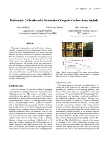
4.2. Exposure EstimationCombining Eq. (2), Eq. (3), and Eq. (18) we have1 1f (Iit ) p0i cos θt qi0 sinθt 0.ktFigure 5. Relationship between lighting, exposures, and image appearance. We need at least two pixel profiles to compute exposuressince many combination of lighting and exposure can result in asame profile.change in the camera. However, there is an inherent ambiguity in computing the exposures from images with different illumination similar to the exponential ambiguity mentioned in the previous section. As can be seen from Eq. (3),there is an infinite number of combinations of the exposureand the lighting that result in the same image intensity. Tocompute the exposure, assumptions on the lighting have tobe made.In this section, we introduce a method to estimate theexposure values given a sequence of images of an outdoorscene taken over a period of time. For the outdoor scenes,the dominant source of lighting is the sun. We model thelighting change according to the motion of the sun and usethe model to compute the exposures. We make the assumption that the sunlight was not blocked by clouds when theimages were taken.4.1. Modeling the Illumination with the Motion ofthe SunThe direction of the sunlight (Lt ) at time t and the surface normal of a point i (Ni ) can be expressed in Cartesiancoordinates as in the following equation where θ’s are theazimuth angles and φ’s are the elevation angles.Lt [cos φt cos θt , cos φt sin θt , sin φt ]TNi [cos φi cos θi , cos φi sin θi , sin φi ]T(16)The lighting due to the sun at point i is thenNi · Lt cos φt cos φi cos(θt θi ) sin φt sin φi (17)Without loss of generality we rotate Lt and Ni so that φt 0, Eq. (17) becomesNi · Lt cos φ0i cos(θt θi0 ) cos φ0i (cos θi0 cos θt sin θi0 sin θt ) pi cos θt qi sin θt(18)where pi cos φ0i cos θi0 and qi cos φ0i sin θi0 . According to Eq. (18), the lighting variation at a point due to thesun over time is a sinusoidal function with the scale and thephase being the parameter.(19)In the above equation, p0i and qi0 are considered to includethe albedo term a from Eq. (3). Additionally, we assumedthat the effect of ambient lighting is constant over time.Note that at least two appearance profiles of different surface normals are necessary to compute the exposures kt ’susing Eq. (19) as shown in Fig. 5.For simplicity, it is assumed that we have a sequence ofη images (1 t η) with pixel values (Iit and Ijt ) of twopoints with different surface normals. From Eq. (19), theexposure kt for each time t is computed by solving a linearleast squares problem Uy 0 with S0η 2 FiU ,(20)0η 2SFj cos θ1 sin θ1 cos θ2 sin θ2 (21)S ,. .cos θη sin θη 1f (Ii1 )0···0 0f 1 (Ii2 ) · · ·0 Fi , (22). 100· · · f (Iiη )y [p1 , q 1 , p2 , q 2 , k10 , k20 , · · · , kη0 ]kt0(23)1 smin2πt( 2460 ),and smin is the samwhere 1/kt , θt pling interval in minutes.A set of pixels used to solve the equation above are randomly selected from the clusters used for the response function estimation (Section 3). It is important not to use pixelvalues at time t in the above equation when the pixels fallinto shadows since the lighting model does not apply toshadow regions. From the appearance profile of a pixel, wedetect whether the pixel is in shadow by a simple thresholding as in [20]. We also remove the pixels from the equationif the average intensity is too low meaning that the pixelswere probably always in the shadow.4.3. Exponential AmbiguityIn Section 3 we discussed the inherent ambiguity in computing the response function where the elements in Eq. (3)are related exponentially as follows.(f 1 (Iit ))γ ktγ aγi Mitγ(24)We resolved this exponential ambiguity by arbitrarily fixingthe scale of the response function which is not a problem
Figure 7. Response function estimation result for Sony SNCRZ30N PTZ cameraFigure 6. Simulation of the effect of the exponential ambiguity.The exposures and the lighting changes were estimated on the twosynthetically generated image profiles similar to Fig. 5 using 400minutes of data (top) and 200 minutes of data (bottom). The correct γ is 1.0.for applications that require image intensity alignment sincedifferent γ’s still result in the same intensity value. Howeverthe arbitrary scale causes problems in methods that requireaccurate or linearly proportional photometric measurementssuch as photometric stereo or motion blur simulation as in[1]. It also affects our exposure estimation process since ourmethod is based on having the right scale for the responsefunction f . If the scale of the response function is incorrect,then the system is trying to fit a sine function to a measurement that is the exponent of a sine. As shown in [4], priorknowledge about the response function f or k (also a orM in our case) is necessary to find the right γ value. Ideally, the error kUyk in Section 4.2 gives us the informationabout the γ. It should be the minimum when the correctscale of the response function is used. However, the erroris not distinctive due to image noise and lack of time interval when surfaces of different normals are both in the sunlight as shown in Fig. 6. Alternatively, we need informationabout the camera or the scene to find the right scale. In thispaper, we first estimate the exposures (kt ) and the lightingfunctions (p0i cos θt qi0 sinθt in Eq. 19) using multiple γvalues. The recovered lighting functions will have differentphases with different γ’s as shown in Fig. 6. We select theγ value that yields the lighting functions to have the peaksat the right time of the day which can be inferred from theorientations of shadows in the image sequence.5. ExperimentsWe first evaluate our response function estimationmethod introduced in Section 3. Two cameras used for theexperiments are Sony SNC-RZ30N PTZ camera and PointGrey Dragonfly camera. For the Sony camera, we first computed the response function by using the method introducedin [8] with multiple images of a static scene with constantillumination to test our method. We then computed the re-Figure 8. Response function estimation result for Point Grey Dragonfly camera with two images used for our estimation.sponse function with our method using four images shownin Fig. 2 and the comparison of the computed response functions is shown in Fig. 7. While only the green channel wasused for this example, we can easily combine all channels ifnecessary. For the Point Grey Dragonfly camera, we compare our result computed with two images with the knownlinear response function which is shown in Fig. 8. The number of images for accurate estimation depends on the intensity range of each image. While the method does not needa large number of points, it is important to have a well distributed pixel intensities for an accurate estimation.To evaluate our exposure estimation method, werecorded images of a scene every minute for a little morethan 4 hours with the Point Grey camera when we couldobserve surfaces with different normals being illuminatedby the sun. Some sample images as well as some of thepixel profiles used for the estimation are shown in Fig. 9.Our exposure estimates are compared to the ground truthexposures reported by the camera in Fig. 10. Notice that theexposure estimates start to deviate from the ground truthstarting around 1400. The cause for this is the change inambient lighting as a building in front of the scene started toblock the sunlight at that time. Since our method is based onconstant ambient lighting, the change in the ambient lighting caused errors in the exposure estimation. However, fora long periods time when the ambient lighting was close toconstant, our estimation was accurate as shown in the figure. We can observe the function of the auto-exposure from
Figure 9. Exposure Estimation. (Top) Sample images from the input sequence and the pixel profiles of the dotted points (Bottom) Imagesand profiles normalized to a fixed exposure. The 0 values in the profiles represent shadow.Figure 11. Estimated response function (left) and the exposures(right) using dataset introduced in [6] (Fig. 12)Figure 10. Comparison of the estimation with the ground truth exposurepixel values vary gradually as expected.6. ConclusionFig. 9. The camera adjusts to the brightness change by trying to fix the intensity of dominant pixels constant. Thisfunction prohibits images from being under-exposed or saturated as can be seen from the exposure compensated images in the figure. While this is good for viewing, this couldaffect vision algorithms that rely on photometric measurements since the image intensities do not reflect true radiance of the points. By computing the response function andexposures using our method, we can convert the image intensities to their actual radiance enabling further analysis ofthe scene.As our last experiment, we used one of the webcamdatasets introduced in [6] as shown in Fig. 12. The imageswe used were captured every 30 minutes for 11 hours. Theestimated response function and the exposures are shown inFig. 11. Note that we do not have the ground truth for thisdata since the camera is unknown. We can roughly evaluate the results by comparing the input images and the pixelprofiles with the images and the profiles normalized withthe estimated exposures as in Fig. 12. Input profiles tendto stay constant unless affected by shadows. However, afternormalizing the images with the estimated exposures, theWe have introduced a novel method for computing thecamera response function for outdoor image sequences inwhich the illumination is changing. This is a challengingproblem because the image appearance varies due to thechanges in both the exposure of the camera and the lighting. Most previous methods cannot deal with the illumination change and the methods that deal with the change arerestrained to some special cases [12, 18]. Our approach alsocomputes the exposure values of the camera with the illumination in the scene changing and we believe this work canserve as a basis for more exciting outdoor scene analysisapplications.For the future, we would like to extend our method tofind the right scale of the response function automatically.One possibility would be using high-order correlations inthe frequency domain such as in [2]. We also plan to enhance our algorithm to take into account the change inambient lighting as well as the change in lighting due toweather. Additionally, we would also like to expand ourmethod to use images from commodity photo collectionssuch as in [19] and [3] which can be used for texture alignment and also help improve image matching.
Figure 12. (Top) Sample images from one of the dataset introduced in [6] and the pixel profiles of the dotted points. (Bottom) Images andprofiles normalized to a fixed exposure. The right side of the figure is to the east.AcknowledgmentsWe gratefully acknowledge the support of the NSF Career award IIS 0237533 as well as a Packard Fellowship forScience and Technology.References[1] P. Debevec and J. Malik. Recovering high dynamic range radiance maps from photographs. Proc. SIGGRAPH’97, pages369–378, Aug. 1997. 2, 6[2] H. Farid. Blind inverse gamma correction. IEEE Transactionon Image Processing, 10(10):1428–1433, 2001. 7[3] M. Goesele, N. Snavely, B. Curless, and S. M. S. H. Hoppe.Multi-view stereo for community photo collections. Proc.IEEE Int. Conf. on Computer Vision, 2007. 7[4] M. Grossberg and S. Nayar. Determining the camera response from images: What is knowable? IEEE Transactionon Pattern Analysis and Machine Intelligence, 25(11):1455–1467, 2003. 2, 4, 6[5] M. Grossberg and S. Nayar. Modeling the space of cameraresponse functions. IEEE Transaction on Pattern Analysisand Machine Intelligence, 26(10):1272–1282, 2004. 2, 4[6] N. Jacobs, N. Roman, and R. Pless. Consistent temporal variations in many outdoor scenes. Proc. IEEE Conference onComputer Vision and Pattern Recognition, pages 1–6, 2004.1, 2, 7, 8[7] N. Jacobs, S. Satkin, N. Roman, R. Speyer, and R. Pless. Geolocating static cameras. Proc. IEEE Int. Conf. on ComputerVision, 2007. 1, 2[8] S. J. Kim and M. Pollefeys. Robust radiometric calibration and vignetting correction. IEEE Transaction on PatternAnalysis and Machine Intelligence, 30(4):562–576, 2008. 2,6[9] S. J. Koppal and S. G. Narasimhan. Clustering appearancefor scene analysis. Proc. IEEE Conference on Computer Vision and Pattern Recognition, pages 1323 – 1330. 3[10] S. Lin, J. Gu, S. Yamazaki, and H. Shum. Radiometric calibration from a single image. Proc. IEEE Conference uter Vision and Pattern Recogni
Radiometric Calibration with Illumination Change for Outdoor Scene Analysis Seon Joo Kim 1Jan-Michael Frahm Department of Computer Science 1University of North Carolina at Chapel Hill sjkim,jmf@cs.