Transcription
Biostatistics 140.754Advanced Methods in Biostatistics IVJeffrey LeekAssistant ProfessorDepartment of Biostatisticsjleek@jhsph.edu1 / 66
Course InformationIWelcome.IThe primary focus of this course is regression modeling, alongwith other more “modern” approaches for estimating orpredicting the relationship between random variables.IThe prerequisites for this course are Biostatistics140.751-140.753.IAll learning outcomes, syllabus, motivation, grading, etc. areavailable from the course website:www.biostat.jhsph.edu/ jleek/teaching/2011/574Lecture notes will be posted the night before class.IICourse evaluation will consist of a weekly reading assignment,a biweekly homework assignment, and a final project.2 / 66
Course Information - CreditsKen Rice (UW) - (slides with a † are directly lifted from himJon Wakefield (UW)Brian Caffo (JHU) Assorted others as mentioned in the text. Any mistakes, typos,or otherwise misleading information is “measurement error” due tome.3 / 66
What’s So Great About Applied Statistics?“I keep saying the sexy job in the next ten years will bestatisticians. People think I’m joking, but who would’ve guessedthat computer engineers would’ve been the sexy job of the 1990s?”- Hal Valarian (Google Chief Economist)4 / 66
“Applied Statisticians”Eric LanderSteven Levi2Nate SilverDaryl MoreyDirector – ton Rockets GM5 / 66
“Jobs For Applied Statisticians”6 / 66
Course Information - How does 574 fit in?†574 is an advanced, Ph.D. level course. The following areassumed:ILinear algebra; expressions like (XT X) 1 XT Y should makesense to you.IIntroductory probability; manipulation of distributions,Central Limit Theorem, Laws of Large Numbers, somelikelihood theoryIIntroductory Regression; some familiarity with multipleregression will be helpfulIThe R Language; sufficient to implement the material above(and look up new stuff in help files)Please note: much of 574 will interpret regression from anon-parametric point of view. This is a modern approach, and maydiffer from classical material you have seen elsewhere.7 / 66
Course Information - How does 574 fit in?574 is a methods courseIThe main aim is to understand how/why methods work andwhat practical situations where they will be most useful.IFormal math will be limited in the lecture notes (unlike in673-674, 771-772), so expect some hand-waving (e.g.“.under mild regularity conditions”).IMany of the course example will be short/stylized. However,the goal of the course is to provide both understanding ofspecific methods and theirimplementation/application/interpretation.8 / 66
Course Information - How does 574 fit in?†The term “methods” is somewhat open to interpretation - this isone potential way to break journals down to give some insightITheory: Annals of Statistics, JRSSB, Statistica SinicaIData Analysis: JASA A&CS, JRSSC, Nature, NEJM, JAMA,Neuroimage, Genome BiologyIMethods: Biometrics, Annals of Applied Statistics,Biostatistics, Statistics in Medicine, Neuroimage, GenomeBiologyModern methods papers use simulation studies to illustratestatistical properties; we will often do the same.Most PhD theses “resemble” methods papers, and contain materialsimilar to that discussed in 574. A focus of this course will bereading, understanding, and learning to construct academic papers.9 / 66
Course Info - TextbooksThere is no fixed textbook for this course. A couple of usefulbooks may be:Modern Applied Statistics with SGeneralized Linear ModelsResearch papers will be featured, for more recent topics - 574 ismore cutting edge than some other courses we teach.10 / 66
Course Info - TextbooksAnother couple of “classics” applied statisticians should haveaccess to:Elements of Statistical LearningAnalysis of Longitudinal DataAn Introduction to the Bootstrap11 / 66
More Ridiculously Useful BooksAnother couple of really useful books - not 100% related to coursecontent, but highly recommendedA course in large sample theory1The Elements of Stylehttp://www.biostat.jhsph.edu/ 1The instructor’s favorite statistics book12 / 66
Course Info - Course ContentIReview of ideas behind regressionINon-parametric inference (generalized method of moments)ILikelihood Quasi-Likelihood inferenceIBayesian inferenceIAnalysis of correlated data - generalized estimating equationsIBootstrappingIModel selection/shrinkage (Lasso, etc.)IFactor analysis/principal components analysisIInteraction-based approaches to prediction/association (i.e.CART)IMultiple testing13 / 66
Outline of Today’s LectureIBackground (randomness, parameters, regression)IRegression with estimating equationsISandwich estimators of variance14 / 66
Terminology†III2The response variable will be termed the outcome. Usually wewish to relate the outcome to covariates.YX (or Z, U)Abbreviation2Preferred nameOutcomeCovariate(s)Other names:Response Regressors, PredictorsOutputInputEndpointExplanatory VariableConfusing Name DependentIndependentPredictor has causal connotations. [In]dependent is a poorchoice (the covariates need not be independent of each other- and may be fixed, by an experimenter)In 574 we consider Y and X which are continuous, categorical,or counts; later in the course multivariate outcomes are brieflyconsidered (more on that in 755/56). Outcomes which arecensored or mixed (e.g. alcohol consumption) are alsopossible. Categorical variables may be nominal or ordinal.Preferred by me15 / 66
What is Randomness?†You may be used to thinking of the stochastic parts of randomvariables as just chance. In very select situations this is fine;radioactive decay really does appear to be just chance 3However, this is not what random variables actually represent inmost applications, and it can be a misleading simplication tothink that its just chance that prevents us knowing the truth.To see this, consider the following thought experiments.3But ask Brian Caffo about this.16 / 66
What is Randomness?†Recall high school physics. For two resistors“in series”, the resistances are added to give atotal (Y , measured in Ohms, Ω) which werecord without errorWe know the number of gold stripes (X) andsilver stripes (Z ). We also know that eachresistance is number of stripes.Q. How much resistance do stripes of eachcolor correspond to?17 / 66
What is Randomness?†Thought experiment #1; Notethat in this situation there no“measurement error” or “noise”,and nothing random is going on.What is the “value” of eachgoldstripe?18 / 66
What is Randomness?†Thought experiment #1; Notethat in this situation there no“measurement error” or “noise”,and nothing random is going on.What is the difference between Xand X 1?19 / 66
What is Randomness?†Thought experiment #1; Notethat in this situation there no“measurement error” or “noise”,and nothing random is going on.What is the difference between Xand X 1?20 / 66
Thought Experiment Math†Here’s the truth;Yn 1 γ0 1n 1 γ1 Xn 1 γ2 Zn 1where n is evenly distributed between all X , Z combinations.But not knowing Z , we will fit the relationshipY β0 1 β1 XHere “fit” means that we will find e orthogonal to 1 and X suchthatY β0 1 β1 X eBy linear algebra (i.e. projection onto 1 and X) we must have Y · (X X̄1)Y · (X X̄1)Y·1 X 1 Xe Y n(X X̄1) · (X X̄1)(X X̄1) · (X X̄1) where X̄ X · 1/(1 · 1) X · 1/n, i.e. the mean of X - a scalar.21 / 66
Thought Experiment Math?†The fitted line, with eNote the orthogonality to 1 and XWhat’s the slope of the line?22 / 66
Thought Experiment Math?†What to remember (in “real” experiments too);IThe “errors” represent everything that we didn’t measure.INothing is random here - we just have imperfect informationIIf you are never going to know Z (or can’t assume you know alot about it) this sort of “marginal” relationship is all that canbe learnedWhat you didn’t measure can’t be ignored.23 / 66
Thought Experiment #2†A different “design”What is going on?24 / 66
Thought Experiment #2†Plotting Y against X ;25 / 66
Thought Experiment #2†Plotting Y against X ;. and not knowing Z26 / 66
Thought Experiment #2†Here’s the fitted line;. what’s the slope?What would you conclude?27 / 66
Thought Experiment #2†Here’s the truth, for both Y and Z;Y γ0 1 γ1 X γ2 ZZ θ0 1 θ1 X where is orthongal to 1, X. Therefore,Y γ0 γ1 X γ2 (θ0 θ1 X ) (γ0 γ2 θ0 )1 (γ1 γ2 θ1 )X γ2 β0 1 β1 X eand we get β1 γ1 if (and only if) there’s “nothing going on”between Z and X . The change we saw in the Y X slope (from#1 to #2) follows exactly this pattern.28 / 66
Thought Experiment #2†IThe marginal slope β1 is not the “wrong” answer, but it maynot be the same as γ1 .IWhich do you wnat? The Y Z slope if Z is fixed or if Zvaries with X in the same way it did in your experiment?INo one needs to know that Y is being measured for β1 6 γ1to occur.IThe “observed” e are actually γ2 here, so the “noise”doesn’t simply reflect the Z X relationship alone29 / 66
Thought Experiment #3†A final “design”. a real mess!30 / 66
Thought Experiment #3†A final “design”. plotting Y vs. X31 / 66
Thought Experiment #3†A final “design”. plotting Y vs. X(Starts to look like real data!)32 / 66
Thought Experiment #3†IZ and X were orthogonal - what happened to the slope?IBut the variability of Z depended on X . What happened to e,compared to #1 and # 2? We can extend all thesearguments to Xn p and Zn q - see Jon Wakefield’s book formore. Reality also tends to have 1 “un-pretty” phenomenaper situation!In general, the nature of what we call “randomness” dependsheavily on what is going on unobserved. Its only in extremelysimple situations4 that unobserved patterns can be dismissedwithout careful thought. In some complex situations they canbe dismissed, but only after careful thought.4.which probably don’t require a PhD statistician33 / 66
Reality Check†This is a realistically- complex“system” you might see in practiceYour “X” might be time(developmental) and “Y”expression of a particular geneKnowing the Y-X relationship isclearly useful, but pretending thatall the Z -X relationships arepretty is naı̈ve (at best)34 / 66
Reality Check†With reasonable sample size n, inference (i.e. learning about β) ispossible without making strong assumptions about the distributionof Y , and how it varies with X. It seems prudent to avoid theseassumptions as “modern” approaches do.IIf you have good a priori reasons to believe them,distributional assumptions may be okay and may helpsubstantiallyIFor small n this may be the only viable approach (other thanquitting)IFor tasks other than inference (e.g. prediction) assumptionsmay be needed.IChecking distributional assumptions after you’ve used themdoesnt actually work very well. Asking the data “was I rightto trust you just now” ? or “did you behave in the way I hopeyou did?” is not reliable, in general.35 / 66
Reality Check†If you have to start making distributional assumptions:IAdding lots of little effects Normal distributionsIBinary events Bernoulli, and BinomialICounting lots of rare events PoissonIContinual (small) hazard of an event Weibull. but note these are rather stylized, minor modications breakthem, e.g. different event rates overdispersed Poisson.However, methods which use classical assumptions often haveother interpretations. For example, using Ȳ (the sample mean) asan estimator can be motivated with Normality, but we don’t needthis assumption in order to use Y .36 / 66
What is a parameter?†From previous courses you will be used to this kind of plot. and also used to “manipulating” the sample in several ways37 / 66
What is a parameter?†You may have seen larger sample sizes,. this sample can also be “manipulated”38 / 66
What is a parameter?†To define parameters, think of an infinite “super”-population;. and consider (simple) ways to manipulate what we see;39 / 66
What is a parameter?†The mean of X;(note: requires finite moments of X to be well-defined)40 / 66
What is a parameter?†The mean of Y ;. mild regularity conditions also apply41 / 66
What is a parameter?†The mean of Y at a given value of X. only sensible if you know the given value of X (!)42 / 66
What is a parameter?†Difference in mean of Y , between two values of X;. which is unchanged, if Y Y c43 / 66
Defining parameters†A parameter is (formally) an operation on a super-population,mapping it to a “parameter space” Θ, such as R, or Rp , or {0, 1}.The parameter value (typically denoted β or θ) is the result of thisoperation5 .I“Inference” means making one or more conclusions about theparameter valueIThese could be estimates, intervals, or binary (Yes/No)decisionsI“Statistical inference” means drawing conclusions withoutthe full populations’ data, i.e. in the face of uncertainty.Parameter values themselves are fixed unknowns; they are not“uncertain” or “random” in any stochastic sense.In previous courses, parameters may have been defined as linearoperations on the superpopulation. In 754, we will generalize theidea.5The “true state of Nature” is a common expression for the same thing44 / 66
Defining parameters†In this course, we will typically assume relevant parameters can beidentified in this way. But in some real situations, one cannotidentify θ, even with an infinite sample (e.g. mean height ofwomen, when you only have data on men)If your data do not permit useful inference, you could;I Switch target parametersI Extrapolate cautiously i.e. make assumptionsI Not do inference, but “hypothesis-generation”I Give upI will mainly disucss “sane” problems; this means ones we canreasonably address. Be aware not every problem is like this.The data may not contain the answer. The combination of somedata and an aching desire for an answer does not ensure that
Biostatistics, Statistics in Medicine, Neuroimage, Genome Biology Modern methods papers use simulation studies to illustrate statistical properties; we will often do the same. Most PhD theses \resemble" methods papers, and contain material similar to that discussed in 574. A focus of this course will be reading, understanding, and learning to construct academic papers. 9/66. Course Info .