Transcription
Compressive Sensing based Single-Pixel Hyperspectral CameraLiang ShiStanford UniversityShihkar ShresthaStanford Abstractlocations) or highly compressible in some basis, relativelyfew incoherent observations will be enough to reconstructa close estimation of the signal. The CS theory provides asensing framework for sampling sparse or compressible signals in a more efficient way that is usually done with Shannon Nyquist sampling scheme. One natural implementationarena of CS theory is the field of imaging.Borrowing idea from this theory, we propose a HS imager that records the light signal with a single detection element, however, without acquiring spectrum of each pixelsquentially. Instead of scanning, a digital micromirror device(DMD) randomly but controllably modulates the lightfrom the scenes which is then summed before reaching thedetector. Since it optically realizes the random measurements described in CS theory, we can use far fewer observations than the total number of pixels to recover the entiredatacube. As a result, it dramatically decreases the data acquisition time and space for data storage. In addition, theintensity of the compressed signal at the detector is muchgreater with respect to raster scan and therefore results ingreater signal sensitivity.In particular, we make the following technical contributions:In this report, we propose a novel compressive hyperspectral(HS) imaging approach which extends the singlepixel camera structure to be applicable for acquiring hyperspectral data. We build a hardware prototupe usingmodified DLP based spatial light modulator, OceanOpticsUSB4000-VIS-NIR spectrometer and Lumencor fiber coupled light engine. We also design an ADMM based reconstruction algorithm and show successful recovery of HS images on both synthetic and real-captured data. In addition,we simulate the HS image reconstruction using spectrometer measurements plus RGB image which gives a more accurate and edge-preserved result under same measurementrate.1. IntroductionHyperspectral(HS) image is 3D datacube storing the intensity of light as a function of wavelength λ at each spatiallocation (x, y). The spectrum distribution revealled by thehyperspectral image is useful in identifying the composition and structure of objects and the environment lightings.Many real applications have been widely used in agriculture, mineralogy, surveillance and so on.In order to capture 3D HS image, conventional approaches always require some form of temporal scanningin either spatial domain or spectral domain. A dispersivepushbroom slit spectromter simultaneously acquires a slitof spatial information, as well as spectral information corresponding to each spatial point in the slit for one scan. Capturing the entire datacube relies on spatial motion of eitherthe spectrometer or the object. A tunable spectral filter imager takes multiple images of the same scene sequentiallyin different bandpass settings. As a result, all these methodsrequire a relatively long acquisition time and huge amountof space for data storage due to the full measurement.Recently, a new theory known as compressive sensing(CS) has emerged. The basic idea of this theory is whenthe signal of interest is very sparese(i.e. zero-valued at most We proposed an extended single-pixel camera structure for capturing HS image using modified DLP projecter, USB4000-VIS-NIR portable spectrometer, andLumencor fiber coupled light engine. We introduce an ADMM based reconstruction algorithm for solving the sparse-constrained optimizationproblem. We give simulation result on 5 different measurement matrices with 5 different priors. Though theoretically simulated by previous papers, weare by far the first group build up the hardware prototype and successfully reconstruct the HS image fromreal-captured data. We simulate the HS image reconstruction using spectrometer measurements plus RGB image, and show itgives a more accurate and edge-preserved result undersame measurement rate.1
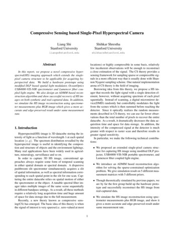
Figure 1. Single-pixel cameraFigure 3. Demonstration of two different measurementsthe weighted sum of all the coded slices along λ-axis. Later,the SD-CASSI[3] architecture is developed by removing thefirst dispersive arm in DD-CASSI. It sacrifices the spectralmultiplexing in DD-CASSI in exchange for the spatial multiplexing. Meanwhile, it reduces the optical elements inthe entire system. In 2011, a DMD-SSI[4] system cameup by replacing the coded aperture with the DMD. Whenreconstructing with multiple shots, DMD-SSI can introduce more randomness, whereas previous approaches onlyprovide a shifted patterns. In 2014, Xing Lin proposed aspatial-spectral encoded snapshot spectral imager[5] whichachieves spatial-spectral modulation by simpliy putting acoded mask between the spectral plane and CCD sensor inhis architecture.Another concept of CS based HS imaging system, whichis also the one implemented in our report, is proposed in [6]at 2009. Fig. 2 shows the difference between this methodwith single-pixel camera. Basically, it extends the singlepixel camera structure by replacing the photodiode with aspectrometer probe. In this architecture, the spatial information is encoded and parallelly measured as the spectralcurve. However, this two and a half pages COSI paper doesnot give any illustration for the hardware setup and reconstruction algorithm. Thus, in our project, all the hardwareprototype and reconstruction algorithms are designed fromscratch.Figure 2. Single-pixel hyperspectral camera2. Related WorkIn 2006, Rice University brought up the first implementation of CS for imaging — the single-pixel camera[1]. It’shardware setup is showed in Fig. 1. With the help of biconvex lens, the desired image is first projected to on theDMD plane. At the same time, a random pattern is generated on the DMD by controlling the state( 12 degrees or-12 degrees) of electrostatically actuated micromirrors. Allthe “on” micromirrors redirect the lights through the secondbiconvex lens which focuses the coded image onto the photodiode. For each random pattern, the photodiode will yieldan absolute voltage measurement as the summed intensityof all the pixels in coded image. If the desired image hassize N w h, by taking M measurements that M N ,we can still reconstruct the gray image with the sparse priors.Recently, a series of CS based snapshot HS imaging systems have been proposed[2,3,4,5,6]. In 2007, amethod called dual-disperser coded aperture snapshot spectral imager(DD-CASSI)[2] first introduced the CS into HSimaging. In the DD-CASSI architecture, the light is spectrally sheared by the first prism, then coded by the mask onaperture, finally unsheared by the second prism. The measurements is captured by a 2D CCD array which records3. ModelIn this section, we will mathematically formulate ourdata capturing process. In addition, we provide a detailedillustration of how CS playing its role in this task by generalizing all the measurements into a sparse-contrained optimization problem.3.1. Spectrometer MeasurementFig. 3 gives an intuitive demonstration of how the datais captured along two different dimensions. First, let’s focus on the spectrometer measurements. Assume the grouth2
truth data G has size RW H S , where W H is the image size and S is the total number of slices along λ. Let{g1 , g2 , . . . , gS } be the images at each slice and m be thetotal number of measurements. We can mathematically represent the acquisition of spectrometer measurements in thefollowing steps:smoothness. As neighbour slices will be similar to eachother, the iterations to convergence will dramatically decrease(almost 50 %). However, since the entire datacubeis decomposed into slices, sparse priors like 3DTV becomeimpossible to fit in this form. In addition, the gray(or RGB)image measurement is also unable to add in the form sinceit has to be expressed as the weighted sum of all the slices.Thus, we give the second and more concept-coherent formulation which reconstructs the datacube at once, initialize i 1 generate an RW H mask Mi using certain rules(i.e.random binominal)s.t. A X B 0min HX 1 ,X Multiply Mi element-wisely with {g1 , g2 , . . . , gS } toobtain the coded images {ci1 , ci2 , . . . , ciS } x1 x2 X . , . xS For each of {ci1 , ci2 , . . . , ciS }, sum the all the elements inside to obtain the single pixel observation{oi1 , oi2 , . . . , oiS } i i 1, repeat until i m Notice, measurements from spectrometer are the summation of pixel values in spatial domain not in spectral domain. b1 b2 B . bS Q A .A . W1 W 2 · · · wi wi Wi . .To impose constraint on spectral dimension, we can capture an RGB image for the target scene. It can be simulatedby applying CIE function to the hyperspectral datacube. Forthe time limitation, we simulate a more simplified versionwhich takes the weighted sum of all the slices to generatea gray image. However, the basic idea is similar and it exerts the same effect as the RGB image. Here, we denote{w1 , w2 , ., wS } as the weights for each slice and Q as anRW H 1 column vector reshaped by the gray image we capture. (4)(5)wiHere, Wi is an Rmatrix with all diagonal elementsequal to wi . This formulation incorporates the gray imagemeasurement and we can remove that by deleting the Wrow in A and Q in B. In both formulations, the underdetermined equations can be solved by finding the sparsestsolution in certain sparese domain and it is also known asthe sparse priors.In our simulation, we implement five different measurement matrices with 5 different sparse priors,Now, we have both spectrometer measurements and grayimage. If we only use the measurements from spectrometer, there are two ways to put all the data into a compressivesensing feasible form. Since the parameters in the first expression will be the building blocks in the second, we introduce that first,xj A WS n n3.3. CS Formulationmin Hxj 1 ,(3) A 3.2. RGB measurement(2)Sensing Matrixs.t. Axj bj 0, j {1, 2, . . . , S} (1)1. random binomialm nHere, A is the an Rmatrix with n W H. It isformed by stretching each Mi into a row vector and stackingall of them vertically. bj is an Rm 1 column vector formedby stacking all oij vertically. xj is an Rn 1 column vectorreshaped by gj .In this expression, the datacube reconstruction is partitioned into several individual problems as reconstructingeach slice by slice. One advantage of solving in this formis we can initialize the guessing of next slice with previous reconstructed one which is reasonable for the spectral2. random Guassian3. permutated DCT4. permutated DFT5. permutated discrete Walsh-Hadamard transformSparse Priorsa. isotropic 2D TV(total variation)3
b. anisotropic 2D TVExcept from isotropic TV, all the other sparese priors try tominimize the L1 norm of wi . Notice, the update is separablewith respect to each wi , so the minimizer ofc. DCTd. wavelet(haar)Tmin wi 1 νi,k(Di uk wi ) wie. 3D TVβi Di uk wi 222(11)is given by 1D shrinkage-like formula,4. ADMM based Reconstructionwi,k 1 max{ Di uk In our project, we use the alternating direction methodof multipliers(ADMM) to solve the sparse-constrainedoptimization problem. Since equation (1) and (2) try tooptimize the same kind of problem with only difference inthe matrices size, we rewrite the problem with different annotations to eliminate the ambiguity of using either of them.1νi,kνi,k , 0}sgn(Di uk )βiβiβi(12)In isotropic TV, we actually minimize the L2 norm of wi ,the minimizer ofTmin wi 2 νi,k(Di uk wi ) minuX Di u ,s.t. Au bwi(6)minwi ,u wi ,wi,k 1 max{ Di uk min LA (wi,k 1 , u) Xuiwi ,uT( wi,k 1 νi,k(Di u wi,k 1 ) iµβi Di u wi,k 1 22 ) Au b 2222its corresponding augmented Lagrangian function is,Xνi,k1Di uk νi,k /βi , 0}βiβi Di uk νi,k /βi (14)Next, we use wi,k 1 to update uk 1 ass.t. Au b and Di u wi for all i (7)min LA (wi , u) (13)is given by 2D shrinkage-like formula,iHere, the term we try to minimize is defined as a summationof u’s norm in several sparse basis, it is considered for thesparse priors like anisotropic TV which consists of firstderivative along both X-axis and Y -axis (and λ-axis in3DTV). Now, we consider the equivalent variant of (3),Xβi Di uk wi 222( wi νiT (Di u wi ) (15)which is equivalent toiµβi Di u wi 22 ) Au b 2222(8)minuThe ADMM solves this problem by sequentially updatingeach parameter while fixing the others. In our problem,each iteration consists of 3 steps as updating wi , u, ν respectively.Assume uk , wi,k and νi,k are the approximate minimizers of (5) at the kth iteration. We first update wi,k 1 byXβiT( νi,k(Di u wi,k 1 ) Di u wi,k 1 22 )2iµ Au b 22 (16)2Notice, it’s a quadratic function and its gradient isdk (u) X(βi DiT ( Di u wi,k 1 ) DiT νi,k )i µAT (Au b) (17)min LA (wi , uk ) wiXT( wi νi,k(Di uk wi ) By setting the gradient to zero, we can obtain the exact minimizer,iβiµ Di uk wi 22 ) Auk b 2222(9)! u k 1which is equivalent to Xβi DiT DiT µA Ai!XXβiTmin( wi νi,k(Di uk wi ) Di uk wi 22 )wi2i(DiT νi,k βi DiT wi,k 1 ) µAT b(18)iwhere the denotes the pseudoinverse of matrix. In practice, it is computationally intractable to compute the inverse(10)4
matrix is feasible at that scale because we only need to turnon few pixels(i.e. 20) for each mask to get a good result.All the combinations are expressed using symbols assignedin section 3.3.(i.e. (1,a) (random binomial, isotropic 2DTV))or pseudoinverse even for the image with a comparativelysmall size(i.e. 128 128). Instead, we adopt one-step gradient descent to get an approximate minimizeruk 1 uk αk dk(19)where αk can be determined by Barzilai and Borweinmethod[7], which suggestsαk (uk uk 1 )T (uk uk 1 )(uk uk 1 )T (dk dk 1 s show one-step gradient descent has good astringency and can dramatically speed up the calculation.Since pixel value in an image should be greater than zero,we perform non-negative projection for all the elements inu after every update,uk 1 max(uk 1 , 0)(21)Finally, we update the multipliers which is trivial comparing with previous stepsνi,k 1 νi,k βi (Di uk 1 wi,k 1 )(22) uk isWe keep updating until the relative change uk 1 uk sufficiently small. The final u will be our best estimationfor the sparse-contrained optimization problem.Combo5. Simulation Result(1,a)(5,a)In this section, we exhaustively evaluate the reconstruction result using simulated data and try to gain someon insight how to choose the parameters to achieve bestreconstruction result.Combo(1,a)(5,a)Experiment 1In the first experiment, we test all the possible combinationof measurement matrices and sparsity priors. The setting ofexperiment is30% measurementRel Err(%) PSNR(db) CPU .9331.9233.2310.6832.1252.3710% measurementRel Err(%) PSNR(db) CPU time(s)2.5444.6215.487.0135.879.083% measurementRel Err(%) PSNR(db) CPU time(s)6.1236.9120.1211.2531.8716.65As shown in table, the isotropic 2D TV consistently yieldsthe lowest reconstruction error. At the scale of 512 512,random binomial measurement matrix with isotropic TVgives the highest PSNR. However, random Guassian matrixhas been proved with best RIP properties and we test itat the scale of 128 128 which does give slightly higheraccuracy. However, the random binomial matrix is the onlyone that otpically feasible. Use “Balloon” set from Columbia Multispectral ImageDatabase Only reconstruct a single slice(thus no 3DTV prior) no image downsamplingExperiment 2In this experiment, we focus on reconstructing the entiredatacube. As mentioned, in the first formulation, we canaccelerate the reconstruction by initializing the guessing ofcurrent slice with previously reconstructed one. Now, weshow the comparison between this strategy with randomguessing initialization on reconstructing 512 512 31datacube. In addition, we also test the reconstruction usingthe second formulation. For all the strategies, we runexperiments on the “Beads” data with 10% measurement. measurement rate: 30%, 10%, 3% no additive noise no test on random Guassian matrix; 20 activated positions for each row of random binomial matrixNotice, we do not test on random Guassian matrix at theoriginal scale since multiplication with it takes O(N 2 )which is intractable when N 5122 . The random binomial5
Figure 4. Result of (1,a) with 3% measurementFigure 7. Result of 2D TV with 10% measurement gray imageFigure 5. Result of (1,a) with 10% measurementFigure 8. Result of 3D TV with 10% measurement gray imageFor the first formulation, we test two different initializtionswith combo (1,a). For the second, we test (1,a) and (1,e)with both random initializtion(cannot pre-initialize). Werun experiments for 5 times, and the results shown beloware the averaged performance. For fair comparison, we donot count the time for generating the measurement matrix.strategy(1,a) & guessing(1,a) & pre-init(1,a) & formulation 2(1,e) & formulation 2Rel Err(%)33.3733.3214.1418.52CPU time(s)402.4168.6250.24255.68As shown, using pre-initializtion dramatically decreases thecalculation time and produces similar result. On the otherhand, with the additional contraint imposed by gray image, the reconstruction results produced by formulation 2Figure 6. Result of (1,a) with 30% measurement6
Figure 11. White light spectrum referenceFigure 9. Result of 2D TV with 10% measurementis originally designed for light projection and consists ofa light engine that integrates RGB LEDs and projection optics. To convert it into a light collector, we remove the LEDsand also the dichroic mirrors to prevent clipping of the spectrum. In addition, we installed a collimating lens (74-series)made by Ocean Optics with a 10mm focal length to direct asmuch light as possible into the fiber (400um core diameter),which couples the light into the spectrometer.Ocean Optics USB4000 UV-VIS spectrometer is used inthe setup for its portability and compatibility with MATLAB. The spectrometer supports the spectrum from 200850 nm, however, the coating on DMD limits the system tooperate in visible range(400-650 nm).To capture hyperspectral data, we also need a powerfullight source that emits light in the entire spectral range of interest. The Lumencor fiber coupled light engine is used forthis setup and configured to approximate a broad band whitelight source. The settings for different LEDs are shown below:Figure 10. Left: modified; Right: originalget a hugh improve which is equivalent to the one obtainedby 30% measurement and only spectrometer measurement.Notice, the performance of 3DTV is worse than 2DTV,it may caused by the excessive smoothing effect imposedalong the λ-axis. We can mitigate this effect by tuning theweight for this sparse component. Violet - 1006. Prototype Blue - 1006.1. Hardware Setup Cyan - 53To verify our model, we build up the hardware setup forcapturing real data. There are three core components in oursetup: spatial light modulator(SLM), spectrometer and lightsource. The basic idea is to light up the scene, use SLM toturn on specfic pixels in the sence and redirect them to thespectrometer, which will measure the spectrum distribution. Teal - 100 Green - 21 Red - 22As shown in the Fig. 10, we modify the TI LightCrafter4500 to be our SLM since it consists of a DMD and control electronics in an integrated development platform. ItFig. 11 shows the white light spectrum captured by thespectrometer in above settings with 20% on-pixels on theDMD.7
Figure 12. Setup in view calibration modeFigure 14. Spectrometer measurement & fitted curveFigure 15. Target sceneimage also requires less measurements under same measurement rate. Here, the integration time we use for eachmeasurement is 150ms. The measurement rate is 50%.Figure 13. Setup in data acquisition mode6.2. Data Capture6.3. Data preprocessingBefore capturing the data, we first need to calibrate thescene to determine the field of view. Fig. 12 showns thesetup in view calibration mode. It is done by coupling thelight into DMD and adjusting the scene to be fully illuminated by the light projected from the LightCrafter. Meanwhile, we upload some random coded masks to examine ifthe DMD works normally.Once we determine the field of view, the light source canbe used to illuminate the scene and the fiber optic connectorfor the spectrometer is connected to the lens for data acquisition. Fig. 13 showns the setup in data acquisition mode.In practice, we turn off the room illumination to proventbackground noise. During the measurement, we generaterandom patterns in MATLAB and switch the DMD basedon the intergration time of spectrometer.In our experiment, we use 600 600 sub-region on theDMD. Every 20 20 pixels are combined to be a superpixel,which leads to a 30 30 image. This operation allows morelights to come in the spectrometer, thus decreases the integration time for each measurement. The low resolutionEach measurement from the spectrometer is stored astwo 3648 1 vectors with one representing the wavelength,the other representing the intensity. As shown in the Fig.14, the captured raw data is very noisy, thus we have tofit a curve for those points. Here, we use smooth functionin MATLAB with smoothing factor equals to 0.1. The fitted curve is also shown in Fig. 14. After that, we take 26samples from 400-650 nm with every 10 nm. By dividingthem with the white reference intensity respectively, we obtain the pre-processed measurement for the reconstructionalgorithm.7. Result from Real-dataWe choose 2D TV as the sparse prior for reconstructingthe real-data. The target scene and reconstruction result areshown in Fig. 15 and Fig. 16 respectively. As shown, allthe colors on the checkerboard are correctly reconstructed.Though the image resolution is low, we can clearly identify the boundaries between each blocks. Fig. 17 shows the8
[2] Gehm M E, John R, Brady D J, et al. Single-shot compressive spectral imaging with a dual-disperser architecture[J]. Optics Express, 2007, 15(21): 14013-14027.[3] Wagadarikar A, John R, Willett R, et al. Single disperser design for coded aperture snapshot spectralimaging[J]. Applied optics, 2008, 47(10): B44-B51.[4] Wu Y, Mirza I O, Arce G R, et al. Developmentof a digital-micromirror-device-based multishot snapshot spectral imaging system[J]. Optics letters, 2011,36(14): 2692-2694.Figure 16. Reconstruction result[5] Lin X, Liu Y, Wu J, et al. Spatial-spectral encoded compressive hyperspectral imaging[J]. ACM Transactionson Graphics (TOG), 2014, 33(6): 233.[6] Sun T, Kelly K. Compressive sensing hyperspectral imager[C]//Computational Optical Sensing and Imaging.Optical Society of America, 2009: CTuA5.[7] Barzilai J, Borwein J M. Two-point step size gradientmethods[J]. IMA Journal of Numerical Analysis, 1988,8(1): 141-148.Figure 17. Spectrum curvespectral curve recovered for the yellow, red and blue blocks.All the peaks show up at the correct wavelength. Since wedo not have the low-resolution ground-truth, we did not calculate the relative error. The result will definitely worsethan the simulation due to the noise from the light source,spectrometer, data fitting and so on. Nevertheless, we arethe first group optically realized the single-pixel hyperspectral camera.8. Future Work and ConclusionIn the future, we want to integrate the RGB camera intoour setup and use its measurement to further improve thereconstruction quality. For the original prototype, we wantto solve the low light issue by finding more powerful andfull-band light source. To reduce the frame capture time, wecan optimize the DMD switching by preloading the patternsonto the board. By solving previous issues, we may try toreconstruct image with higher resolution.References[1] Duarte M F, Davenport M A, Takhar D, et al. Singlepixel imaging via compressive sampling[J]. IEEE Signal Processing Magazine, 2008, 25(2): 83.9
the “on” micromirrors redirect the lights through the second biconvex lens which focuses the coded image onto the pho-todiode. For each random pattern, the photodiode will yield an absolute voltage measurement as the summed intensity of all the pixels in coded image. If the desired