Transcription
CHAPTER 4EARTH PRESSURETHEORY ANDAPPLICATION
EARTH PRESSURE THEORY AND APPLICATION4.0 GENERALAll shoring systems shall be designed to withstand lateral earth pressure, water pressure and theeffect of surcharge loads in accordance with the general principles and guidelines specified in thisCaltrans Trenching and Shoring Manual.4.1 SHORING TYPESShoring systems are generally classified as unrestrained (non-gravity cantilevered), and restrained(braced or anchored). Unrestrained shoring systems rely on structural components of the wallpartially embedded in the foundation material to mobilize passive resistance to lateral loads.Restrained shoring systems derive their capacity to resist lateral loads by their structuralcomponents being restrained by tension or compression elements connected to the verticalstructural members of the shoring system and, additionally, by the partial embedment (if any) oftheir structural components into the foundation material.4.1.1 Unrestrained Shoring SystemsUnrestrained shoring systems (non-gravity cantilevered walls) are constructed of verticalstructural members consisting of partially embedded soldier piles or continuous sheet piles.This type of system depends on the passive resistance of the foundation material and themoment resisting capacity of the vertical structural members for stability; therefore itsmaximum height is limited by the competence of the foundation material and the momentresisting capacity of the vertical structural members. The economical height of this type ofwall is generally limited to a maximum of 18 feet.4.1.2 Restrained Shoring SystemsRestrained Shoring Systems are either anchored or braced walls.They are typicallycomprised of the same elements as unrestrained (non-gravity cantilevered) walls, but deriveadditional lateral resistance from one or more levels of braces, rakers, or anchors. Thesewalls are typically constructed in cut situations in which construction proceeds from the topdown to the base of the wall. The vertical wall elements should extend below the potentialfailure plane associated with the retained soil mass. For these types of walls, economicalwall heights up to 80 feet are feasible.4-1
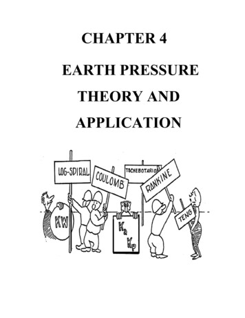
CT TRENCHING AND SHORING MANUALNote - Soil Nail Walls and Mechanically Stabilized Earth (MSE) Walls are not included inthis Manual. Both of these types of systems are designed by other methods that can befound on-line with FHWA or AASHTO.4.2 LOADINGA major issue in providing a safe shoring system design is to determine the appropriate earthpressure loading diagram. The loads are to be calculated using the appropriate earth pressuretheories.The lateral horizontal stresses (σ) for both active and passive pressure are to becalculated based on the soil properties and the shoring system. Earth pressure loads on a shoringsystem are a function of the unit weight of the soil, location of the groundwater table, seepageforces, surcharge loads, and the shoring structure system. Shoring systems that cannot tolerate anymovement should be designed for at-rest lateral earth pressure. Shoring systems which can moveaway from the soil mass should be designed for active earth pressure conditions, depending on themagnitude of the tolerable movement. Any movement, which is required to reach the minimumactive pressure or the maximum passive pressure, is a function of the wall height and the soil type.Significant movement is necessary to mobilize the full passive pressure. The variation of lateralstress between the active and passive earth pressure values can be brought about only throughlateral movement within the soil mass of the backfill as shown in Figure 4-1.Ultimate PassivePassivePpPoPaAt Rest p a aActive pDisplacementToward the backfillAway from the backfillFigure 4-1. Active and passive earth pressure coefficient as a function of wall displacement4-2
EARTH PRESSURE THEORY AND APPLICATIONTypical values of these mobilizing movements, relative to wall height, are given in Table 4-1(Clough 1991).Table 4-1. Mobilized Wall MovementsValue of /HType of BackfillActivePassiveDense Sand0.0010.01Medium Dense Sand0.0020.02Loose Sand0.0040.04Compacted Silt0.0020.02Compacted Lean Clay0.010.05Compacted Fat Clay0.010.05where: the movement of top of wall required to reach minimum active or maximum passivepressure, by tilting or lateral translation, andH height of wall.4-3
CT TRENCHING AND SHORING MANUAL4.3 GRANULAR SOILAt present, methods of analysis in common use for retaining structures are based on Rankine(1857) and Coulomb (1776) theories. Both methods are based on the limit equilibrium approachwith an assumed planar failure surface. Developments since 1920, largely due to the influence ofTerzaghi (1943), have led to a better understanding of the limitations and appropriate applicationsof classical earth pressure theories.Terzaghi assumed a logarithmic failure surface. Manyexperiments have been conducted to validate Coulomb’s wedge theory and it has been found thatthe sliding surface is not a plane, but a curved surface as shown in Figure 4-2 (Terzaghi 1943).Plane SurfaceCurve SurfaceFigure 4-2. Comparison of Plane versus Curve Failure SurfacesFurthermore, these experiments have shown that the Rankine (1857) and Coulomb (1776) earthpressure theories lead to quite accurate results for the active earth pressure. However, for thepassive earth pressure, these theories are accurate only for the backfill of clean dry sand for a lowwall interface friction angle.For the purpose of the initial discussion, it is assumed that the backfills are level, homogeneous,isotropic and distribution of vertical stress (σv) with depth is hydrostatic as shown in Figure 4-3.4-4
EARTH PRESSURE THEORY AND APPLICATIONThe horizontal stress (σh) is linearly proportional to depth and is a multiple of vertical stress (σv)as shown in. Eq. 4-1.σ σ K γ hKEq. 4-11P σh h2Eq. 4-2hvDepending on the wall movement, the coefficient K represents active (Ka), passive (Kp) or at-rest(Ko) earth pressure coefficient in the above equation.The resultant lateral earth load, P, which is equal to the area of the load diagram, shall be assumedto act at a height of h/3 above the base of the wall, where h is the height of the pressure surface,measured from the surface of the ground to the base of the wall. P is the force that causes bending,sliding and overturning in the wall.Figure 4-3. Lateral Earth Pressure Variation with DepthDepending on the shoring system the value of the active and/or passive pressure can be determinedusing either the Rankine, Coulomb, Log Spiral and Trial Wedge methods.The state of the active and passive earth pressure depends on the expansion or compressiontransformation of the backfill from elastic state to state of plastic equilibrium. The concept of theactive and passive earth pressure theory can be explained using a continuous deadman near the4-5
CT TRENCHING AND SHORING MANUALground surface for the stability of a sheet pile wall as shown in Figure 4-4. As a result of walldeflection, , the tie rod is pulled until the active and passive wedges are formed behind and infront of the deadman. Element P, in the front of the deadman and element A, at the front of thedeadman are acted on by two principal stresses, a vertical stress (σv) and horizontal stress (σh). Inthe active case, the horizontal stress (σa) is the minor principal stress and the vertical stress (σv) isthe major principal stress. In the passive case, the horizontal stress (σp) is the major principalstress and the vertical stress (σv) is the minor principal stress. The resulting failure surface withinthe soil mass corresponding to active and passive earth pressure for the cohesionless soil is shownin Figure 4-4.4-6
EARTH PRESSURE THEORY AND APPLICATION TierodPASheet PilewallOFigure 4-4. Mohr Circle Representation of Earth Pressure for Cohesionless Backfill4-7
CT TRENCHING AND SHORING MANUALFrom Figure 4-4 above:σv σasin φ AB2 OA σ v σ a2Eq. 4-3Where AB is the radius of the circleAB σ v σ a OA σ v σ aEq. 4-4σ v sin φ σ a sin φ σ v σ aEq. 4-5sin φ Collecting Terms:σ a σ a (sin φ ) σ v σ v (sin φ )Eq. 4-6σ a (1 sin φ ) σ v (1 sin φ )Eq. 4-7σ a (1 sin φ ) σ v (1 sin φ )Eq. 4-8From trigonometric identities:(1 sinφ ) tan2 45 φ 2 (1 sinφ )(1 sinφ ) tan2 45 φ 2 (1 sinφ ) σK a tan2 45 φ , where K a a2 σvEq. 4-9For the passive case:Kp σ p 1 sin φ tan 2 45 φ 2 σ v 1 sin φEq. 4-10There are various pros and cons to the individual earth theories but briefly here is a summary: The Rankine formula for passive pressure can only be used correctly when theembankment slope angle, β, equals zero or is negative. If a large wall friction value candevelop, the Rankine Theory is not correct and will give less conservative results.Rankine's theory is not intended to be used for determining earth pressures directly againsta wall (friction angle does not appear in equations above). The theory is intended to beused for determining earth pressures on a vertical plane within a mass of soil.4-8
EARTH PRESSURE THEORY AND APPLICATION For the Coulomb equation, if the shoring system is vertical and the backfill slope frictionangles are zero, the result will be the same as Rankine's for a level ground condition. Sincewall friction requires a curved surface of sliding to satisfy equilibrium, the Coulombformula will give only approximate results since it assumes planar failure surfaces. Theaccuracy for Coulomb will diminish with increased depth. For passive pressures theCoulomb formula can also give inaccurate results when there is a large back slope or wallfriction angle. These conditions should be investigated and an increased factor of safetyconsidered. The Log-Spiral theory was developed because of the unrealistic values of earth pressuresthat are obtained by theories that assume a straight line failure plane. The differencebetween the Log-Spiral curved failure surface and the straight line failure plane can belarge and on the unsafe side for Coulomb passive pressures (especially when wall frictionexceeds φ/3). Figure 4-2 and Figure 4-31 show a comparison of the Coulomb and Rankinefailure surfaces (plane) versus the Log-Spiral failure surface (curve). More on Log-Spiral can be found in Section 4.7 of this Manual.4-9
CT TRENCHING AND SHORING MANUAL4.3.1 At-Rest Lateral Earth Pressure Coefficient (K0)For a zero lateral strain condition, horizontal and vertical stresses are related by the Poisson’sratio (µ) as follows:µKo 1 µEq. 4-11For normally consolidated soils and vertical walls, the coefficient of at-rest lateral earthpressure may be taken as:Ko (1 sin φ )(1 sin β )Eq. 4-12Where:φ effective friction angle of soil.Ko coefficient of at-rest lateral earth pressure.β slope angle of backfill surface behind retaining wall.For over consolidated soils, level backfill, and a vertical wall, the coefficient of at-rest lateralearth pressure may be assumed to vary as a function of the over consolidation ratio or stresshistory, and may be taken as:K O (1 sin φ )(OCR )sin φEq. 4-13Where:OCR over consolidation ratio4-10
EARTH PRESSURE THEORY AND APPLICATION4.3.2 Active and/or Passive Earth PressureDepending on the shoring system the value of the active and/or passive pressure can bedetermined using either the Rankine, Coulomb or trial wedge methods.4.3.2.1 Rankine’s TheoryRankine’s theory is the simplest formulation proposed for earth pressure calculations andit is based on the following assumptions: The wall is smooth and vertical. No friction or adhesion between the wall and the soil. The failure wedge is a plane surface and is a function of soil’s friction φ andthe backfill slope β as shown in Eq. 4-14 and Eq. 4-17. Lateral earth pressure varies linearly with depth. The direction of the lateral earth pressure acts parallel to slope of the backfillas shown in Figure 4-5 and Figure 4-6. The resultant earth pressure acts at a distance equal to one-third of the wallheight from the base.Values for the coefficient of active lateral earth pressure using the Rankine Theory maybe taken as shown in Eq. 4-14:cos β cos 2β cos 2φK cos βacos β cos 2β cos 2φEq. 4-14And the magnitude of active earth pressure can be determined as shown in Figure 4-5and Eq. 4-15:( )1Pa (γ ) h2 (Ka )2Eq. 4-15The failure plane angle α can be determined as shown in Eq. 4-16: sin β φ 1 α 45 Arc sin β sin φ 2 2 4-11Eq. 4-16
CT TRENCHING AND SHORING MANUALFigure 4-5. Rankine’s active wedgeRankine made similar assumptions to his active earth pressure theory to calculate thepassive earth pressure. Values for the coefficient of passive lateral earth pressure may betaken as:K p cos βcos β cos 2β cos 2φcos β cos 2β cos 2φEq. 4-17And the magnitude of passive earth pressure can be determined as shown in Figure 4-6and Eq. 4-18:Pp ( )( )1(γ ) h2 K p2Eq. 4-184-12
EARTH PRESSURE THEORY AND APPLICATIONThe failure plane angle α can be determined as shown in Eq. 4-19: sin β φ 1 α 45 Arc sin β sin φ 2 2 Figure 4-6. Rankine’s passive wedge4-13Eq. 4-19
CT TRENCHING AND SHORING MANUALWhere:h height of pressure surface on the wall.Pa active lateral earth pressure resultant per unit width of wall.Pp passive lateral earth pressure resultant per unit width of wall.β angle from backfill surface to the horizontal.α failure plane angle with respect to horizontal.ø effective friction angle of soil.Ka coefficient of active lateral earth pressure.Kp coefficient of passive lateral earth pressure.γ unit weight of soil.Although Rankine’s equation for the passive earth pressure is provided above, one shouldnot use the Rankine method to calculate the passive earth pressure when the backfillangle is greater than zero (β 0). As a matter of fact the Kp value for both positive (β 0)and negative (β 0) backfill slope is identical. This is clearly not correct. Therefore,avoid using the Rankine equation to calculate the passive earth pressure coefficient forsloping ground.4.3.2.2 Coulomb’s TheoryCoulomb’s (1776) earth pressure theory is based on the following assumptions: The wall is rough. There is friction or adhesion between the wall and the soil. The failure wedge is a plane surface and is a function of the soil friction φ,wall friction δ, the backfill slope β and the slope of the wall ω. Lateral earth pressure varies linearly with depth. The direction of the lateral earth pressure acts at an angle δ with a line that isnormal to the wall. The resultant earth pressure acts at a distance equal to one-third of the wallheight from the base.4-14
EARTH PRESSURE THEORY AND APPLICATIONValues for the coefficient of active lateral earth pressure may be taken as shown in Eq.4-20:Ka cos 2(φ ω ) 2δ φφ βsinsin()()cos 2ω cos (δ ω) 1 cos (δ ω )cos (ω β ) Eq. 4-20And the magnitude of active earth pressure can be determined as shown in Figure 4-7and Eq. 4-21:( )1Pa (γ ) h2 (Ka )2Eq. 4-21Figure 4-7. Coulomb’s active wedge4-15
CT TRENCHING AND SHORING MANUALCoulomb’s passive earth pressure is derived similar to his active earth pressure except theinclination of the force is as shown in Figure 4-7. Values for the coefficient of passivelateral earth pressure may be taken as shown in Eq. 4-22:Kp cos 2(φ ω )2 sin(δ φ )sin(φ β ) 2cos ω cos(δ ω) 1 cos(δ ω )cos(β ω ) Eq. 4-22And the magnitude of passive earth pressure can be determined as shown in Figure 4-8and Eq. 4-23:Pp ( )( )1(γ ) h2 K p2Eq. 4-23Figure 4-8. Coulomb’s passive wedge4-16
EARTH PRESSURE THEORY AND APPLICATIONWhere:h height of pressure surface on the wall.Pa active lateral earth pressure resultant per unit width of wall.Pp passive lateral earth pressure resultant per unit width of wall.δ friction angle between backfill material and face of wall.(See Table 4-2)β angle from backfill surface to the horizontal.α failure plane angle with respect to the horizontal.ω angle from the face of wall to the vertical.ø effective friction angle of soil.Ka coefficient of active lateral earth pressure.Kp coefficient of passive lateral earth pressure.γ unit weight of soil.4-17
CT TRENCHING AND SHORING MANUALTable 4-2. Wall frictionULTIMATE FRICTION FACTOR FOR DISSIMILAR MATERIALSFRICTIONANGLE, δ( )INTERFACE MATERIALSMass concrete on the following foundation materials: Clean sound rock · · · · · · · · · · · · · · · · · · · · · · · · · · · · · · · · · · · · · · · · · · · · · · Clean gravel, gravel-sand mixtures, coarse sand· · · · · · · · · · · · · · · · · · · · · · · · Clean fine to medium sand, silty medium to coarse sand, silty or clayey gravel · Clean fine sand, silty or clayey fine to medium sand· · · · · · · · · · · · · · · · · · · · · Fine sandy silt, nonplastic silt · · · · · · · · · · · · · · · · · · · · · · · · · · · · · · · · · · · · · Very stiff and hard residual or preconsolidated clay · · · · · · · · · · · · · · · · · · · · · Medium stiff and stiff clay and silty clay· · · · · · · · · · · · · · · · · · · · · · · · · · · · ·3529 to 3124 to 2919 to 2417 to 1922 to 2617 to 19Masonry on foundation materials has same friction factors.Steel sheet piles against the following soils: Clean gravel, gravel-sand mixtures, well-graded rock fill with spalls· · · · · · · · · Clean sand, silty sand-gravel mixture, single-size hard rock fill· · · · · · · · · · · · · Silty sand, gravel or sand mixed with silt or clay · · · · · · · · · · · · · · · · · · · · · · · Fine sandy silt, nonplastic silt· · · · · · · · · · · · · · · · · · · · · · · · · · · · · · · · · · · · ·Formed or precast concrete or concrete sheet piling against the following soils: Clean gravel, gravel-sand mixture, well-graded rock fill with spalls· · · · · · · · · · Clean sand, silty sand-gravel mixture, single-size hard rock fill· · · · · · · · · · · · · Silty sand, gravel or sand mixed with silt or clay · · · · · · · · · · · · · · · · · · · · · · · Fine sandy silt, nonplastic silt· · · · · · · · · · · · · · · · · · · · · · · · · · · · · · · · · · · · ·2217141122 to 2617 to 221714Various structural materials: Masonry on masonry, igneous and metamorphic rocks:o dressed soft rock on dressed soft rock · · · · · · · · · · · · · · · · · · · · · · · · · · ·o dressed hard rock on dressed soft rock · · · · · · · · · · · · · · · · · · · · · · · · · ·o dressed hard rock on dressed hard rock · · · · · · · · · · · · · · · · · · · · · · · · · · Masonry on wood in direction of cross grain · · · · · · · · · · · · · · · · · · · · · · · · · · Steel on steel at sheet pile interlocks · · · · · · · · · · · · · · · · · · · · · · · · · · · · · · · ·This table is a reprint of Table 3.11.5.3-1, AASHTO LRFD BDS, 4th ed, 2007Further discussion of Wall Friction is included in Section 4.6.4-183533292617
EARTH PRESSURE THEORY AND APPLICATION4.4 COHESIVE SOILNeither Coulomb’s nor Rankine’s theories explicitly incorporated the effect of cohesion in thelateral earth pressure computations. Bell (1952) modified Rankine’s solution to include the effectof the backfill with cohesion. The derivation of Bell’s equations for the active and passive earthpressure follows the same steps as were used in Section 4.3 as shown below.For the cohesive soil Figure 4-9 can be used to derive the relationship for the active and passiveearth pressures.Figure 4-9. Mohr Circle Representation of Earth Pressure for Cohesive BackfillFor the Active case:σ v σ asin φ 2σ v σa2Eq. 4-24c tan φThen,σ v sin φ σ a sin φ 2c (cos φ ) σ p σ aEq. 4-25Collecting Terms:σ v (1 sin φ ) σ a (1 sin φ ) 2c (cos φ )Eq. 4-26Solving for σa4-19
CT TRENCHING AND SHORING MANUALσa σ v (1 sin φ ) 2c (cos φ ) (1 sin φ ) (1 sin φ )Eq. 4-27Using the trigonometric identities from above: 2 2 σ a σ v tan2 45 φ 2c tan 45 φ Eq. 4-28σ a σ v K a 2c K a , where σ v γ zEq. 4-29For the passive case:Solving for σpσp σ v (1 sin φ ) 2c (cos φ ) (1 sin φ ) (1 sinφ ) 2 Eq. 4-30 2 σ p σ v tan 2 45 φ 2c tan 45 φ Eq. 4-31σ p σ v K p 2c K p , where σ v γ zEq. 4-32Extreme caution is advised when using cohesive soil to evaluate soil stresses. The evaluation ofthe stress induced by cohesive soils is highly uncertain due to their sensitivity to shrinkage-swell,wet-dry and degree of saturation. Tension cracks (gaps) can form, which may considerably alterthe assumptions for the estimation of stress. The development of the tension cracks from thesurface to depth, hcr, is shown in Figure 4-10.hcrFigure 4-10. Tension crack with hydrostatic water pressure4-20
EARTH PRESSURE THEORY AND APPLICATIONAs shown in Figure 4-11, the active earth pressure (σa) normal to the back of the wall at depth, h,is equal to:σ a γ h K a 2C K aEq. 4-331Pa γ h 2 K a 2C K a (h )2Eq. 4-34According to Eq. 4-33 the lateral stress (σa) at some point along the wall is equal to zero, therefore,Eq. 4-35γ h K a 2C K a 0h hcr 2C K aγ KaEq. 4-36As shown in Figure 4-11, the passive earth pressure (σp) normal to the back of the wall at depth, h,is equal to:σ p γ h K p 2C K pEq. 4-371Pp γ h 2 K p 2C K p (h )2Eq. 4-38Figure 4-11. Cohesive Soil Active Passive Earth Pressure DistributionThe effect of the surcharges and ground water are not included in the above figure. In the presenceof water, the hydrostatic pressure in the tension crack needs to be considered.4-21
CT TRENCHING AND SHORING MANUALFor shoring systems which support cohesive backfill, the height of the tension zone, hcr, should beignored and the simplified lateral earth pressure distribution acting along the entire wall height, h,including presence of water pressure within the tension zone as shown in Figure 4-12 shall beused.(a) Tension Crack with Water(b) Recommended Pressure Diagram for DesignFigure 4-12: Load Distribution for Cohesive BackfillThe apparent active earth pressure coefficient, Kapparent, may be determined by:K apparent σa 0.25γhEq. 4-39Where: (for Eq. 4-24 through Eq. 4-39)h height of pressure surface at back of wall.Pa active lateral earth pressure resultant per unit width of wall.Pp passive lateral earth pressure resultant per unit width of wall.ø effective friction angle of soil.C effective soil cohesion.Ka coefficient of active lateral earth pressure.Kp coefficient of passive lateral earth pressure.γ unit weight of soil.hcr height of the tension crack.4-22
EARTH PRESSURE THEORY AND APPLICATIONThe active lateral earth pressure (σa) acting over the wall height, h, should not be less than 0.25times the effective vertical stress (σv γh) at any depth. Any design based on a lower value musthave superior justification such as multiple laboratory tests verifying higher values for "C", as wellas time frames and other conditions that would not affect the cohesive value while the shoring is inplace.4-23
CT TRENCHING AND SHORING MANUAL4.5 SHORING SYSTEMS AND SLOPING GROUNDThere are many stable slopes in nature even though the slope angle β is larger than the soil frictionangle φ due to presence of cohesion C. None of the earth pressure theories will work when theslope angle β is larger than friction angle φ even if the shoring system is to be installed in cohesivesoil. Mohr Circle representation of the C-φ soil backfill with slope angle β φ is shown in Figure4-13.Figure 4-13. Sloping GroundThe following equations developed by the authors are based on ASCE Journal of Geotechnical andGeoenvironmental Engineering (February 1997) and are used to solve this problem.csin β sin φ cos φlEq. 4-40Where:l 11 σ x sin(2φ ) σ v (cos β 2 cos φ 2 ) σ x c sin(2φ ) c2 cos φ 2 2cos φ σ γ (H cos β )V[2(σ x γ H cos2 β]Eq. 4-41)The following outlines various methods for analyzing shoring systems that have sloping groundconditions.4-24
EARTH PRESSURE THEORY AND APPLICATION4.5.1 Active Trial Wedge MethodFigure 4-14 shows the assumptions used to determine the resultant active pressure for slopingground with an irregular backfill condition applying the wedge theory. This is an iterativeprocess. The failure plane angle (αn) for the wedge varies until the maximum value of theactive earth pressure is computed using Eq. 4-42. The development of Eq. 4-42 is based on thelimiting equilibrium for a general soil wedge. It is assumed that the soil wedge movesdownward along the failure surface and along the wall surface to mobilize the active wedge.This wedge is held in equilibrium by the resultant force equal to the resultant active pressure(Pa) acting on the face of the wall. Since the wedge moves downward along the face of thewall, this force acts with an assumed wall friction angle (δ) below the normal to the wall tooppose this movement.For any assumed failure surface defined by angle αn from the horizontal and the length of thefailure surface Ln, the magnitude of the wedge weight (Wn) is the weight of the soil wedge plusthe relevant surcharge load.For any failure wedge the maximum value of Pa can bedetermined using Eq. 4-42.Pa [][[][W tan (α φ ) C oLc sin α tan (α φ ) cosα C aL a tan (α φ )cos ( ω ) sin ω1 tan (δ ω ) tan (α φ ) cos (δ ω )]]Eq. 4-424-25
CT TRENCHING AND SHORING MANUALFigure 4-14. Active Trial WedgeWhere:Pa active lateral earth pressure resultant per unit width of wall.W weight of soil wedge plus the relevant surcharge loads.δ friction angle between backfill material and back of wall.ø effective friction angle of soil.αn failure plane angle with respect to horizontal.C soil cohesion.Ln length of the failure plane.4-26
EARTH PRESSURE THEORY AND APPLICATION4.5.2 Passive Trial Wedge MethodFigure 4-15 shows the assumptions used to determine the resultant passive pressure for abroken back slope condition applying the trial wedge theory. Using the limiting equilibriumfor a given wedge, Eq. 4-43 calculates the passive earth pressure on a wall. The same iterativeprocedure is used as was used for the active case. However, the failure surface angle (αn) isvaried until the minimum value of passive pressure Pp is attained.Pp [][[][W ta n (α φ ) C oL c sin α ta n (α φ ) c os α C aL a tan (α φ )cos ( ω ) sinω1 tan (δ ω )tan (α φ ) c os (δ ω )]]Eq. 4-43Figure 4-15. Passive Trial Wedge4-27Revised August 2011
CT TRENCHING AND SHORING MANUALWhere:Pp passive lateral earth pressure resultant per unit width of wall.Wn weight of soil wedge plus the relevant surcharge loads.δ friction angle between backfill material and back of wall.ø effective friction angle of soil.αn failure plane angle with respect to horizontal.C soil cohesion.Ln length of the failure plane.4.5.3 Culmann’s Graphical Solution for Active Earth PressureCulmann (1866) developed a convenient graphical solution procedure to calculate the activeearth pressure for retaining walls for irregular backfill and surcharges. Figure 4-16 shows afailure wedge and a force polygon acting on the wedge. The forces per unit width of the wallto be considered for equilibrium of the wedge are as onTensionCrack ProProffile-PaCaHWCBCaωPaα(α- φ)RWCφDSingle WedgeFigure 4-16. Single Wedge and Force Polygon4-28Force Polygon
EARTH PRESSURE THEORY AND APPLICATION1. W Weight of the wedge including weight of the tension crack zone and the surchargeswith a known direction and magnitudeW ABDEFA(γ ) q(lq ) VareaEq. 4-442. Ca Adhesive force along the backfill of the wall with a known direction and magnitudeC c (BD)aEq. 4-453. C Cohesive force along the failure surface with a known direction and magnitudeC c (DE)Eq. 4-464. ho Height of the tension crack2 C Kaφ ho ; Where Ka tan2 45 2 g (Ka )Eq. 4-475. R Resultant of the shear and normal forces acting on the failure surface DE with thedirection known only6. Pa Active force of wedge with the direction known onlyWhere:c Soil cohesion value.Ka Rankine active earth pressure coefficient.φ Soil friction angle.γ Unit weight of soil.To determine the maximum active force against a retaining wall, several trial wedges must beconsidered and the force polygons for all the wedges must be drawn to scale as shown Figure4-17.4-29
CT TRENCHING AND SHORING MANUALGBackfillProfileKV2AETensionCrack ProfileWCaHBhon 2Cnωn 1nM1qFφPaαnRnCritical WedgeDTrial WedgesFigure 4-17. Culmann Trial WedgesThe procedure for estimating the maximum active force, Pa, as shown in Figure 4-17and Figure 4-18, is described as follows:1.Draw the lines for the tensile crack profile parallel to the backfill profile withheight equal to ho.2.Draw several trial wedges to intersect the tension crack profile line.3.Draw the vectors to represent the weight of wedges per unit width of the wallincluding the surcharges.4.Draw adhesion force vector Ca acting along the face of the wall.5.Draw cohesion force vector Coh acting along the failure surfaces.6.Draw the active force vector Pa.7.Draw the resultant force vector R acting on the failure place8.Repeat steps 2 through 7 until all trial wedges are complete4-30
EARTH PRESSURE THEORY AND APPLICATION9.Draw a smooth curve through these points as shown in Figure 4-18. A cubicspline function is used in CT-Flex computer program to draw the smooth linebetween point P1 through point Pn 2 as shown in Figure 4-18.10.Draw dashed line TT’ through the left end of force vectors Pa as shown in Figure4-18.Draw a parallel line to line TT’ that is tangent to the above curve to measuremaximum active earth pressure length as shown in Figure 4-18.12.Draw a line parallel to the force vectors Pa that begins at TT’ and ends at theintersection point of the tangent line to the curved line above.maximum active pressure force vector Pamax.The maximum active pressure shown in Figure 4-17 and Figure 4-18 is obtained as:Pa (length of L) x (load
Ultimate PassivePassive Away from the backfill. . transformation of the backfill from elastic state to state of plastic equilibrium. The concept of the active and passive earth pressure theory can be explained using a co